Making Fun Algebra Problems Funner October 29th, 2010
Patrick Stein

A month ago, a friend posted the following problem on Facebook. I just noticed it this week.
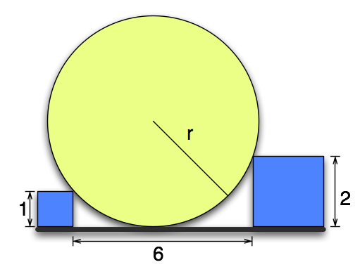
Drawing of a circle with radius r sitting on a line with two squares wedged against it.  One square has side-length 1, the other side-length 2.  There are six units between the squares.
The goal is to find the exact length of the radius r.

I love this kind of math problem.  It has a bunch of features that make it a great, toy math problem.

  • It looks like it’s going to be easy, but at the same time seems at a glance to not have enough information
  • It looks like a geometry problem but only requires that you know:
    • All radii of a circle have the same length
    • A radius to a point where a tangent line touches the circle is perpendicular to that tangent line
  • It requires only very basic algebra:
    • Pythagorean theorem
    • Solving quadratics
  • The numbers in the problem are small, non-zero integers

I spent the next 25 minutes and six pieces of paper working the problem. About 20% of the time that I spent was rechecking my work. Why did I bother rechecking my work on a toy problem?

Warning: Spoilers ahead. If you like this kind of problem, stop reading now and play with it first.

The problem with the problem

This problem failed to satisfy one of my other criterion for great, toy puzzle problems.

  • The answer is a small natural number (or the current year)

I am notorious for messing up signs when doing large algebra calculations. I had to check and recheck all of my work to make sure that I hadn’t done 5x - (3x - 2) and gotten 2x - 2 somewhere. If I had come up with an integer value for r, I’d have been done. Instead, the answer involved a half-integer plus a multiple of \sqrt{74}.

What? \sqrt{74}?!? Raise your hand if you’ve ever seen that written anywhere before this problem.

That’s what I thought.

So, I spent the next hour looking for a different set of numbers to put in for 1, 2, and 6 so that the radius r would come out to an integer. My approach was Brownian, at best. I threw Pythagorean triples at a wall until one stuck.

The sticky triple left me with [50,200,360] to put in place of [1,2,6]. So, I put the problem down for awhile.

The next time that I was in the car, I realized that the radius for the sticky triple was less than 200. That meant that the larger box was touching the upper half of the circle instead of the lower half. The circle had to overlap the box.

So, I was back to the drawing board. Of course, I’d have been back to the drawing board at some point anyway because that sticky triple violated both of my small numbers criteria.

Warning: If you want to play around with finding a set of numbers that work, do it before you read the following. There are even more spoilers ahead.

Infinitely many combinations to get an integer radius

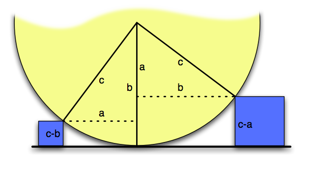
When I next sat down to play (pronounced: /OBSESS/) with this problem, I quickly hit upon the following way to take any Pythagorean triple (a, b, c) and make a version of the above puzzle where the radius r is an integer.
Same sort of diagram as above except radius is c, boxes are height c-b and c-a, and some (a,b,c) triangles are drawn in

In fact, using a 3-4-5 triangle, it is obvious that had the distance between the blocks in the original problem been 7 instead of 6, the radius would have been a small natural number.

Now. Now, I had infinitely many ways to construct this problem so that the radius was an integer. But, did I have all of the ways?

All your configuration are belong to us

When looking at that last diagram, the first question that comes to mind (for me) is: Do I really need to use the same Pythagorean triple on the left and right triangles? The answer, of course, is No.

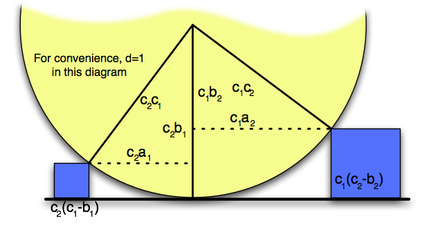
If I have two Pythagorean triples (a_1,b_1,c_1) and (a_2,b_2,c_2) and d is any (positive) divisor of both c_1 and c_2, then I can start with an a_1-b_1-c_1 triangle on the left and an a_2-b_2-c_2 triangle on the right. I can then scale up the left triangle by c_2/d and scale the right triangle up by c_1/d. Now, both triangles have the same hypotenuse.

This means that if the left block has height c_2 (c_1 - b_1)/d, the right block has height c_1(c_2 - b_2)/d, the distance between the two blocks is (c_2 a_1 + c_1 a_2)/d, and the resulting circle has radius c_1c_2/d.
A more general version of the previous diagrams

Does this cover all of the solutions? Could I possibly have non-integer a_1 and a_2 such that (c_2a_1 + c_1a_2)/d is still integer?

Well, for the problem to be formulated entirely with integers, we certainly need the hypotenuse of the right triangles to be an integer. Further, to make the blocks integer heights then both of the legs of the right triangles along the vertical radius must also be integer. So, if the triangle on the left had hypotenuse r, vertical leg b and horizontal leg a, then we know that a = \sqrt{r^2 - b^2} where both r and b are integers. Thus, a must be the square root of an integer.

It is easy to see that if a were a non-integer rational number, then its square would also be a non-integer rational number. So, either a is integer or it is the irrational square root of an integer.

So, can a be an irrational number? If a were an irrational number, then the horizontal leg of the other triangle would have to be some integer n minus the irrational a for the distance between the two blocks to be an integer. Let’s say the vertical leg of the triangle on the right is \beta. Just like b in the first triangle, \beta must be an integer. We also know that (n-a)^2 = r^2 - \beta^2. This, in turn, means that a = (\beta^2 + n^2 + a^2 - r^2) / (2n). The right hand side is clearly rational, so a could not have been irrational.

So, there you have it: all of the numbers that make this problem have all integers on the drawing and an integer answer.

Finding the Perfect Hyperbola February 15th, 2010
Patrick Stein

For an application that I’m working on, I needed a way to scale quantities that range (theoretically) over the real numbers (though practically are probably between plus and minus three) into positive numbers. I wanted the function to be everywhere increasing, I wanted f(0) = 1, and I wanted control of the derivative at x = 0.

The easy choice is: f(x) = e^{\alpha x}. This is monotonically increasing. f(0) = 1 and f^\prime(0) = \alpha.

I needed to scale three such quantities and mush them together. I thought it’d be spiffy then to have three different functions that satisfy my criteria. The next logical choice was f(x) = 1 + \mathrm{tanh} (\alpha x). It is everywhere positive and increasing. And, it has f^\prime(0) = \alpha.

Now, I needed third function that was always positive, always increasing, had f(0) = 1 and f^\prime(0) = \alpha. One choice was: f(x) = e^{e^{\alpha x} - 1}. But, that seemed like overkill. It also meant that I really had to keep my \alpha tiny if I didn’t want to scale things into the stratosphere.

Playing with hyperbolas

So, I thought… why don’t I make a hyperbola, rotate it, and shift it so that the apex of one side of the hyperbola is at (0,1). And, I can adjust the parameters of the hyperbola so that f'(0) = \alpha. After a variety of false starts where I tried to keep the hyperbola general until the very end (\frac{x^2}{a^2} - \frac{y^2}{b^2} = r^2, rotated by \theta degrees, and shifted by \beta), I quickly got bogged down in six or seven incredibly ugly equations in eight or nine variables.

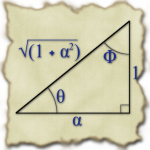
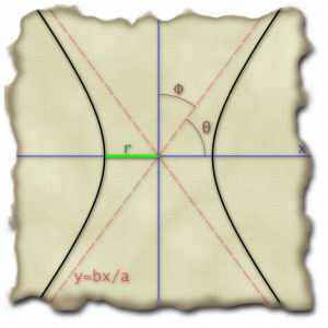
So, it was time to start trying to make it easy from the beginning. I noticed that if was going to rotate it by an angle \theta in the clockwise direction, then I needed \phi = \frac{\pi}{2} - \theta to be such that \tan \phi = \alpha if my slope was going to work out right in the end. So, I’m looking at the basic triangle on the right then to determine all of my sines and cosines and such.

Based on that triangle, it was also obvious that the asymptote for my starting hyperbola had to have \frac{b}{a} = \frac{1}{\alpha}. I played around a bit then with making a = \alpha and b = 1. In the end, I found things simplified sooner if I started with a = 1 and b = \frac{1}{\alpha}.

I also needed r to be such that the point (-r,0) rotate up so that its y-coordinate was 1. This meant that r \sin \theta = 1 or r = \frac{1}{\sin \theta} = \sqrt{1 + \alpha^2}.

So, my starting hyperbola then was: x^2 - \alpha^2 y^2 = 1 + \alpha^2.

From there, I had to rotate the x and y by \theta in the clockwise direction. This gave me:

(x\cos\theta - y\sin\theta)^2 - \alpha^2 (x\sin\theta + y\cos\theta)^2 = 1 + \alpha^2

A little multiplying out leads to:

(x^2\cos^2\theta - 2xy\sin\theta\cos\theta + y^2\sin^2\theta) \\ - \alpha^2(x^2\sin^2\theta + 2xy\sin\theta\cos\theta + y^2\cos^2\theta) = 1 + \alpha^2

From there, using cos^2\theta = \frac{\alpha^2}{1 + \alpha^2}, sin^2\theta = \frac{1}{1 + \alpha^2}, and \sin\theta\cos\theta = \frac{\alpha}{1 + \alpha^2}, we come to:

\frac{-2\alpha(1 + \alpha^2)xy + ( 1 - \alpha^4 )y^2}{1 + \alpha^2} = -2\alpha{}xy +  (1 - \alpha^2)y^2 = 1 + \alpha^2

The only step remaining was to shift it all over so that when y = 1, we end up with x = 0. Plugging in y = 1, we see that -2x\alpha + 1 - \alpha^2 = 1 + \alpha. That equation balances when x = -\alpha. We want it to balance when x = 0, so we’re going to substitute (x - \alpha) in place of the x in the above equation to get:

-2\alpha(x - \alpha)y + (1 - \alpha^2)y^2 = 1 + \alpha^2

We can easily verify that the point (0,1) is on the curve. And, we can implicitly differentiate the above to get:

-2\alpha(x - \alpha)\frac{dy}{dx} - 2\alpha{}y + 2(1 - \alpha^2)y\frac{dy}{dx} = 0

Plopping x = 0 and y = 1 in there, we find that \frac{dy}{dx} = \alpha.

This is pretty good as it goes. The only step is to complete the square to find a nicer expression for y in terms of x. We start by adding \left[ \frac{\alpha}{\sqrt{1 - \alpha^2}} (x - \alpha) \right]^2 to both sides to get:

\left[ \sqrt(1 - \alpha^2)y - \frac{\alpha}{\sqrt{1 - \alpha^2}(x - \alpha)} \right]^2 = 1 + \alpha^2 + \frac{\alpha}{1 - \alpha^2} (x-\alpha)^2

This is easy enough to solve for y by taking the square root of both sides and shuffling some things about:

y = \frac{\alpha}{1 - \alpha^2}(x - \alpha) + \frac{1}{\sqrt{1 - \alpha^2}} \sqrt{1 + \alpha^2 + \frac{\alpha^2}{1 - \alpha^2}(x - \alpha)^2}

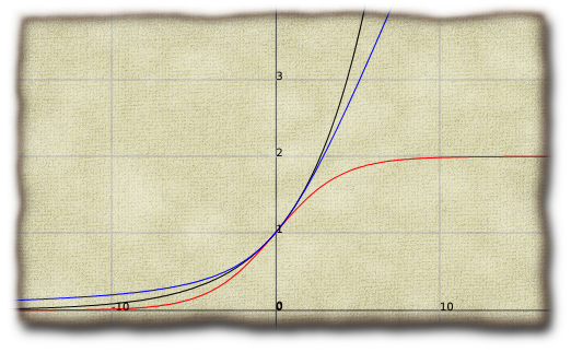
Here are all three curves with \alpha = \frac{1}{4}. The exponential is in black, the hyperbolic tangent is in red, and the hyperbola is in blue:

The first image on the page here was made with Zach’s Vecto library with some post-processing in the GIMP. (Here is the source file: hyperbola.lisp.) The second image was made entirely within the GIMP. And, the last image was made using Foo Plot and the GIMP.

Image Approximation with Genetically Selected Cosines October 2nd, 2009
Patrick Stein

input imageI started with the target image here on the right. I then used a genetic algorithm to try to find an approximation of this image as a sum of cosine waves.

Each cosine wave has the following form

f_i(x,y) = A_i \cos \left( 2 \pi \left( x \cos \theta_i + y \cos \theta_i \right) \omega_i + 2 \pi \phi_i \right)
The genetic algorithm can tweak the amplitude A_i, the orientation in the plane \theta_i, the frequency \omega_i, and the phase \phi_i of each wave.

out-0442 The image at the right here, is from the 443rd generation of a population of 200 where each gene represents 100 cosine waves. For the video below, I used a population of 100 genes, each representing the sum of 50 cosine waves.

Image Approximation with Genetically Selected Cosines from Patrick Stein on Vimeo.

Nitty Gritty Details

The genes are represented internally as an array of fixed-point numbers. Each number is five-bits integer, ten-bits fractional, and a sign bit. I scale the amplitudes down by a factor of 50 and scale the frequency and offset up by 50% when I convert them back to floating point from the fixed point representation just to get them into a more useful ballpark. During each generation, the fittest two quartiles of the population are cross-bred (in randomly selected pairs with two-point crossover) to replace the third quartile of the population, and the fourth quartile is replaced by mutations of randomly selected members of the top quartile. I also run through and remove any duplicate genes and replace them with randomly generated ones so that I don’t breed myself into a total corner.

I toyed around with two different fitness functions: RMS and entropy. So, I would calculate the image represented by the gene and subtract that from the original image. Then, I would calculate the RMS (\frac{\sum_{i=1}^{n} v_i^2}{n}) or the sum of the entropies of the possible values (\sum_{v=0}^{255} - p_v \log p_v, where p_v is the proportion of the pixels in the resulting image that had value v).

I bothered with entropy because I was hoping that if I could encode a gene in just a hundred or two hundred bytes that I might be able to compress the remainder (losslessly) and save bytes over just compressing the original image. The big problem with the entropy calculation though is that I get the same answer when every pixel value is off by 100 as I get when every pixel value is right on target. So, for a time, I was multiplying the RMS and the entropy for the fitness function. For the video and images above, I just used the RMS since it reached very close to the same solution as the multiplying method, and I saved myself fifty histograms per generation.

Source Code

Here is the Common Lisp source code for the genetic algorithm. It depends on the CL-PNG library for image input and output. As it appears here, it will create an output image from the fittest member of each generation, an image of the fittest member of the current generation, an image of the original with the fittest member of the current generation subtracted, a Lisp file containing the fittest gene of the current generation, and the current state of the random number generator when the run ends.

For the video above, I quickly put together some code to demonstrate the different parameters that the genetic algorithm can tweak and to show incrementally adding in more of the cosine waves. Here is some general utility code that is display-independent. And, here is the OpenGL display code which depends on the CL-OpenGL libraries. I included the source code here because I had trouble finding an example on the net of using Lisp-created textures with CL-OpenGL. I render the cosine waves into a buffer, copy that buffer into an OpenGL texture, and draw a quad with that texture. Note: it looks a little sluggish when run, but that is because I put a big (SLEEP …) in there to keep things from flying by too quickly.

Fourier Transform of Swarm Data with HUD September 25th, 2009
Patrick Stein

I added a heads-up display to the code from the previous article. This display shows you the coordinates of each of the bees.

The leader-bee is thick white string with green beads. The follower-bees are the thin black strings with red beads. Going clockwise from the top, the beads on each string represent amplitude, x-frequency, y-frequency, x-phase, and y-phase. The outside of the HUD represents positive infinity. The inner circle of the HUD represents negative infinity. The light yellow circle between the infinities represents zero. Note: the scaling is extreme. Two is almost 90% of the way from zero to infinity on this scale.

Fourier Swarm with Bee Display from Patrick Stein on Vimeo.

Technical details of the HUD scaling

Say you have a number m that you want to map into the interval [-1,1]. Draw the upper half of the unit circle centered at the origin. Start moving from left to right along the circle until you find the spot with a tangent of slope m. Use the x-coordinate of this point. To map that interval onto my HUD, subtract your calculated x-coordinate from two and use the result as the radius from the center of the HUD.

Here is the Lisp source code. It depends on Zach’s Vecto library.

Edit: Oops… there is a bug in the HUD code. The leader and first follower are not shown. The second follower is the thick white line. Ooops. Okay… I have replaced the video and the source code now.

Beautiful Random FFTs September 22nd, 2009
Patrick Stein

Neil Baylis emailed me a program he had put together that puts a few random numbers in a grid and does the inverse FFT of them. His program cycles the values placed in the grid between -1 and 1 to animate some different effects. I like just regenerating random ones over and over again or tweaking which cells of the grid are in use. [You may already be on the same page as I am here, but I’ve got an idea kicking around now that I just have to try…. watch for it in a day or two.]

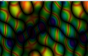
blob_thing Here is one of the nifty designs that I generated with his program. I encourage you to download it and play around a little bit. It is really great to see in real-time how activating certain frequencies affects the output.

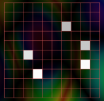
For reference, blob_thing_grid here are the frequencies that I had activated for the above picture.

There are gorgeous specular features and shading in his output images. He could have just it left it flat-colored, but he went the extra distance to add a lighting model. The results are stunning. You should click on the above image to see it full-size. And, you should check out the the example on Neil’s page.


l