Visualizing Galois Fields May 17th, 2012
Patrick Stein

Galois fields are used in a number of different ways. For example, the AES encryption standard uses them.

Arithmetic in Galois Fields

The Galois fields of size 2^n for various n are convenient in computer applications because of how nicely they fit into bytes or words on the machine. The Galois field GF(2^n) has 2^n elements. These elements are represented as polynomials of degree less than n with all coefficients either 0 or 1. So, to encode an element of GF(2^n) as a number, you need an n-bit binary number.

For example, let us consider the Galois field GF(2^3). It has 2^3 = 8 elements. They are (as binary integers) 000, 001, 010, 011, 100, 101, 110, and 111. The element 110, for example, stands for the polynomial x^2 + x. The element 011 stands for the polynomial x + 1.

The coefficients add together just like the integers-modulo-2 add. In group theory terms, the coefficients are from \mathbb{Z}/2\mathbb{Z}. That means that 0 + 0 = 0, 0 + 1 = 1, 1 + 0 = 1, and 1 + 1 = 0. In computer terms, a + b is simply a XOR b. That means, to get the integer representation of the sum of two elements, we simply have to do the bitwise-XOR of their integer representations. Every processor that I’ve ever seen has built-in instructions to do this. Most computer languages support bitwise-XOR operations. In Lisp, the bitwise-XOR of a and b is (logxor a b).

Multiplication is somewhat trickier. Here, we have to multiply the polynomials together. For example, (x + 1) \cdot x = x^2 + x. But, if we did (x^2 + x) \cdot x, we’d end up with x^3 + x^2. We wanted everything to be polynomials of degree less than n and our n is 3. So, what do we do?

What we do, is we take some polynomial of degree n that cannot be written as the product of two polynomials of less than degree n. For our example, let’s use x^3 + x + 1 (which is 1011 in our binary scheme). Now, we need to take our products modulo this polynomial.

You may not have divided polynomials by other polynomials before. It’s a perfectly possible thing to do. When we divide a positive integer a by another positive integer b (with b bigger than 1), we get some answer strictly smaller than a with a remainder strictly smaller than b. When we divide a polynomial of degree m by a polynomial of degree n (with n greater than zero), we get an answer that is a polynomial of degree strictly less than m and a remainder that is a polynomial of degree strictly less than n.

Dividing proceeds much as long division of integers does. For example, if we take the polynomial (with integer coefficients) x^3 + 2x + 5 and divide it by the polynomial x + 3, we start by writing it as:

x + 3 \overline{\left) x^3 + 0x^2 + 2x + 5\right.}
We notice that to get (x+3) \cdot q(x) to start with x^3, we need q(x) to start with x^2. We then proceed to subtract (x+3) \cdot x^2 and then figure out that we need a -3x for the next term, and so on. We end up with x^2 - 3x + 11 with a remainder of -28 (a degree zero polynomial).

\begin{array}{ccrcrcrcr}& & & & x^2 & - & 3x & + & 11 \\& \multicolumn{8}{l}{\hrulefill} \\(x+3) & ) & x^3 & + & 0x^2 & + & 2x & + & 5 \\& & x^3 & + & 3x^2 & & & & \\& & \multicolumn{3}{l}{\hrulefill} & & & & \\& & & - & 3x^2 & + & 2x & & \\& & & - & 3x^2 & - & 9x & & \\& & & \multicolumn{4}{l}{\hrulefill} & & \\& & & & & & 11x & + & 5 \\& & & & & & 11x & + & 33 \\& & & & & & \multicolumn{3}{l}{\hrulefill} \\& & & & & & & - & 28\end{array}
For the example we cited earlier we had x^3 + x^2 which we needed to take modulo x^3 + x + 1. Well, dividing x^3 + x^2 by x^3 + x + 1, we see that it goes in one time with a remainder of x^2 + x + 1. [Note: addition and subtraction are the same in GF(2^n).]

\begin{array}{ccrcrcrcr}& & & & & & & & 1 \\& \multicolumn{8}{l}{\hrulefill} \\(x^3+x+1) & ) & x^3 & + & x^2 & + & 0x & + & 0 \\& & x^3 & + & 0x^2 & + & x & + & 1 \\& & \multicolumn{7}{l}{\hrulefill} \\& & & & x^2 & + & x & + & 1\\\end{array}
For a reasonable way to accomplish this in the special case of our integer representations of polynomials in GF(2^n), see this article about Finite Field Arithmetic and Reed Solomon Codes. In (tail-call style) Lisp, that algorithm for GF(2^8) might look something like this to multiply a times b modulo m:

(flet ((next-a (a)
(ash a -1))
(next-b (b)
(let ((overflow (plusp (logand b #x80))))
(if overflow
(mod (logxor (ash b 1) m) #x100)
(ash b 1)))))
(labels ((mult (a b r)
(cond
((zerop a) r)
((oddp a) (mult (next-a a) (next-b b) (logxor r b)))
(t (mult (next-a a) (next-b b) r)))))
(mult a b 0)))

How is the Galois field structured?

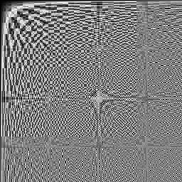
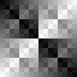
The additive structure is simple. Using our 8-bit representations of elements of GF(2^8), we can create an image where the pixel in the i-th row and j-th column is the sum (in the Galois field) of i and j (written as binary numbers). That looks like this:
Just before the above-mentioned article hit reddit, I got to wondering if the structure of the Galois field was affected at all by the choice of polynomial you used as the modulus. So, I put together some code to try out all of the polynomials of order 8.

Remember way back at the beginning of multiplication, I said that the modulus polynomial had to be one which couldn’t be written as the product of two polynomials of smaller degree? If you allow that, then you have two non-zero polynomials that when multiplied together will equal your modulus polynomial. Just like with integers, if you’ve got an exact multiple of the modulus, the remainder is zero. We don’t want to be able to multiply together two non-zero elements to get zero. Such elements would be called zero divisors.

Zero divisors would make these just be Galois rings instead of Galois fields. Another way of saying this is that in a field, the non-zero elements form a group under multiplication. If they don’t, but multiplication is still associative and distributes over addition, we call it a ring instead of a field.

Galois rings might be interesting in their own right, but they’re not good for AES-type encryption. In AES-type encryption, we’re trying to mix around the bits of the message. If our mixing takes us to zero, we can never undo that mixing—there is nothing we can multiply or divide by to get back what we mixed in.

So, we need a polynomial that cannot be factored into two smaller polynomials. Such a polynomial is said to be irreducible. We can just start building an image for the multiplication for a given modulus and bail out if it has two non-zero elements that multiply together to get zero. So, I did this for all elements which when written in our binary notation form odd numbers between (and including) 100000001 and 111111111 (shown as binary). These are the only numbers which could possibly represent irreducible polynomials of degree 8. The even numbers are easy to throw out because they can be written as x times a degree 7 polynomial.

The ones that worked were: 100011011, 100011101, 100101011, 100101101, 100111001, 100111111, 101001101, 101011111, 101100011, 101100101, 101101001, 101110001, 101110111, 101111011, 110000111, 110001011, 110001101, 110011111, 110100011, 110101001, 110110001, 110111101, 111000011, 111001111, 111010111, 111011101, 111100111, 111110011, 111110101, and 111111001. That first one that worked (100011011) is the one used in AES. Its multiplication table looks like:
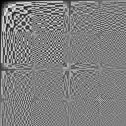
Here’s it is again on the left with the multiplication table when 110011111 is the modulus on the right:

 
So, the addition image provides some insight into how addition works. The multiplication tables, at least for me, provide very little insight into anything. They don’t even make a good stereo pair.

To say two of the multiplication tables have the same structure, means there is some way to map back and forth between them so that the multiplication still works. If we have table X and table Y, then we need an invertible function f such that f(a \cdot_X b) = f(a) \cdot_Y f(b) for all a and b in the table X.

What’s next?

If there is an invertible map between two multiplication tables and there is some element a in the first table, you can take successive powers of it: a, a^2, a^3, \ldots. There are only 2^n elements in GF(2^n) no matter which polynomial we pick. So, somewhere in there, you have to start repeating. In fact, you have to get back to a. There is some smallest, positive integer k so that a^{k+1} \equiv a in GF(2^n). If we pick a = 0, then we simply have that k = 1. For non-zero a, we are even better off because a^k \equiv 1.

So, what if I took the powers of each element of GF(2^n) in turn? For each number, I would get a sequence of its powers. If I throw away the order of that sequence and just consider it a set, then I would end up with a subset of GF(2^n) for each a in GF(2^n). How many different subsets will I end up with? Will there be a different subset for each a?

I mentioned earlier that the non-zero elements of GF(2^n) form what’s called a group. The subset created by the powers of any fixed a forms what’s called a subgroup. A subgroup is a subset of a group such that given any two members of that subset, their product (in the whole group) is also a member of the subset. As it turns out, for groups with a finite number of elements, the number of items in a subgroup has to divide evenly into the number of elements in the whole group.

The element zero in GF(2^n) forms the subset containing only zero. The non-zero elements of GF(2^n) form a group of 2^n - 1 elements. The number 2^n - 1 is odd (for all n \ge 1). So, immediately, we know that all of the subsets we generate are going to have an odd number of items in them. For GF(2^8), there are 255 non-zero elements. The numbers that divide 255 are: 1, 3, 5, 15, 17, 51, 85, and 255.

It turns out that the non-zero elements of GF(2^n) form what’s called a cyclic group. That means that there is at least one element a whose subset is all 2^n - 1 of the non-zero elements. If take one of those a‘s in GF(2^8) whose subset is all 255 of the elements, we can quickly see that the powers of a^3 form a subset containing 85 elements, the powers of a^5 form a subset containing 51 elements, …, the powers of a^{85} form a subset containing 3 elements, and the powers of a^{255} form a subset containing 1 element. Further, if both a and b have all 255 elements in their subset, then a^k and b^k will have the same number of elements in their subsets for all k. We would still have to check to make sure that if a^i + a^j = a^k that b^i + b^j = b^k to verify the whole field structure is the same.

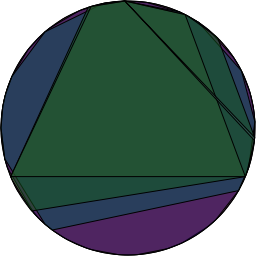
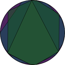
This means there are only 8 different subset of GF(2^8)‘s non-zero elements which form subgroups. Pictorially, if we placed the powers of a around a circle so that a^0 = 1 was at the top and the powers progressed around the circle and then drew a polygon connecting consecutive points, then consecutive points in the a^3 sequence and consecutive points in the a^5 sequence, etc…. we’d end up with this:
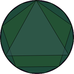
If we don’t reorder them and just leave them in the numerical order of their binary representation, the result isn’t as aesthetically pleasing as the previous picture. Here are the same two we used before 100011011 (on the left) and 110011111 (on the right). They are easier to look at. They do not lend much more insight nor make a better stereo pair.

 
*shrug* Here’s the source file that I used to generate all of these images with Vecto and ZPNG: group.lisp

Finding the Perfect Hyperbola February 15th, 2010
Patrick Stein

For an application that I’m working on, I needed a way to scale quantities that range (theoretically) over the real numbers (though practically are probably between plus and minus three) into positive numbers. I wanted the function to be everywhere increasing, I wanted f(0) = 1, and I wanted control of the derivative at x = 0.

The easy choice is: f(x) = e^{\alpha x}. This is monotonically increasing. f(0) = 1 and f^\prime(0) = \alpha.

I needed to scale three such quantities and mush them together. I thought it’d be spiffy then to have three different functions that satisfy my criteria. The next logical choice was f(x) = 1 + \mathrm{tanh} (\alpha x). It is everywhere positive and increasing. And, it has f^\prime(0) = \alpha.

Now, I needed third function that was always positive, always increasing, had f(0) = 1 and f^\prime(0) = \alpha. One choice was: f(x) = e^{e^{\alpha x} - 1}. But, that seemed like overkill. It also meant that I really had to keep my \alpha tiny if I didn’t want to scale things into the stratosphere.

Playing with hyperbolas

So, I thought… why don’t I make a hyperbola, rotate it, and shift it so that the apex of one side of the hyperbola is at (0,1). And, I can adjust the parameters of the hyperbola so that f'(0) = \alpha. After a variety of false starts where I tried to keep the hyperbola general until the very end (\frac{x^2}{a^2} - \frac{y^2}{b^2} = r^2, rotated by \theta degrees, and shifted by \beta), I quickly got bogged down in six or seven incredibly ugly equations in eight or nine variables.

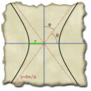
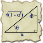
So, it was time to start trying to make it easy from the beginning. I noticed that if was going to rotate it by an angle \theta in the clockwise direction, then I needed \phi = \frac{\pi}{2} - \theta to be such that \tan \phi = \alpha if my slope was going to work out right in the end. So, I’m looking at the basic triangle on the right then to determine all of my sines and cosines and such.

Based on that triangle, it was also obvious that the asymptote for my starting hyperbola had to have \frac{b}{a} = \frac{1}{\alpha}. I played around a bit then with making a = \alpha and b = 1. In the end, I found things simplified sooner if I started with a = 1 and b = \frac{1}{\alpha}.

I also needed r to be such that the point (-r,0) rotate up so that its y-coordinate was 1. This meant that r \sin \theta = 1 or r = \frac{1}{\sin \theta} = \sqrt{1 + \alpha^2}.

So, my starting hyperbola then was: x^2 - \alpha^2 y^2 = 1 + \alpha^2.

From there, I had to rotate the x and y by \theta in the clockwise direction. This gave me:

(x\cos\theta - y\sin\theta)^2 - \alpha^2 (x\sin\theta + y\cos\theta)^2 = 1 + \alpha^2

A little multiplying out leads to:

(x^2\cos^2\theta - 2xy\sin\theta\cos\theta + y^2\sin^2\theta) \\ - \alpha^2(x^2\sin^2\theta + 2xy\sin\theta\cos\theta + y^2\cos^2\theta) = 1 + \alpha^2

From there, using cos^2\theta = \frac{\alpha^2}{1 + \alpha^2}, sin^2\theta = \frac{1}{1 + \alpha^2}, and \sin\theta\cos\theta = \frac{\alpha}{1 + \alpha^2}, we come to:

\frac{-2\alpha(1 + \alpha^2)xy + ( 1 - \alpha^4 )y^2}{1 + \alpha^2} = -2\alpha{}xy +  (1 - \alpha^2)y^2 = 1 + \alpha^2

The only step remaining was to shift it all over so that when y = 1, we end up with x = 0. Plugging in y = 1, we see that -2x\alpha + 1 - \alpha^2 = 1 + \alpha. That equation balances when x = -\alpha. We want it to balance when x = 0, so we’re going to substitute (x - \alpha) in place of the x in the above equation to get:

-2\alpha(x - \alpha)y + (1 - \alpha^2)y^2 = 1 + \alpha^2

We can easily verify that the point (0,1) is on the curve. And, we can implicitly differentiate the above to get:

-2\alpha(x - \alpha)\frac{dy}{dx} - 2\alpha{}y + 2(1 - \alpha^2)y\frac{dy}{dx} = 0

Plopping x = 0 and y = 1 in there, we find that \frac{dy}{dx} = \alpha.

This is pretty good as it goes. The only step is to complete the square to find a nicer expression for y in terms of x. We start by adding \left[ \frac{\alpha}{\sqrt{1 - \alpha^2}} (x - \alpha) \right]^2 to both sides to get:

\left[ \sqrt(1 - \alpha^2)y - \frac{\alpha}{\sqrt{1 - \alpha^2}(x - \alpha)} \right]^2 = 1 + \alpha^2 + \frac{\alpha}{1 - \alpha^2} (x-\alpha)^2

This is easy enough to solve for y by taking the square root of both sides and shuffling some things about:

y = \frac{\alpha}{1 - \alpha^2}(x - \alpha) + \frac{1}{\sqrt{1 - \alpha^2}} \sqrt{1 + \alpha^2 + \frac{\alpha^2}{1 - \alpha^2}(x - \alpha)^2}

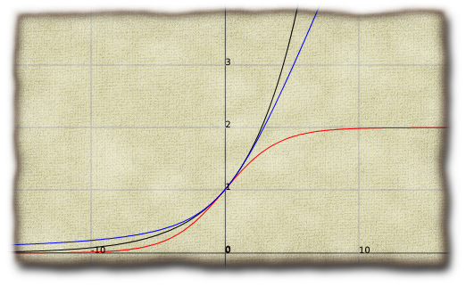
Here are all three curves with \alpha = \frac{1}{4}. The exponential is in black, the hyperbolic tangent is in red, and the hyperbola is in blue:

The first image on the page here was made with Zach’s Vecto library with some post-processing in the GIMP. (Here is the source file: hyperbola.lisp.) The second image was made entirely within the GIMP. And, the last image was made using Foo Plot and the GIMP.

DSL for Drawing Floor Plans October 28th, 2009
Patrick Stein

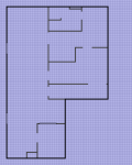
Last week, I needed create a scale drawing of my basement floor plan. My license for OmniGraffle Professional are long since out-of-date. I didn’t want to pay $200 for a new license or even another $75 if I can dig up one of my old license keys. So, what’s a hacker to do? Roll his own (on top of Zach’s Vecto library).

My first cut worked, but was pretty ugly:

(with-floor-plan #P"basement.png" 200.0
   (interior-wall :start (cons (- 91 31 1/2) 0) ; hose cover
                  :north 18
                  :east  (+ 31 1/2))
   (interior-wall :start (cons 91 (- 103 27 30)) ; storage wall
                  :south (- 103 27 30))
   (interior-wall :start (cons (+ 91 83) 103)  ; fish-tank wall
                  :to '(91 . 103)
                  :south 27)
   ...)

basement
I ended up with large calculations like that (- 103 27 30) you see there. It worked. I got an okay looking floor-plan out of it. But, it was obvious that it needed some rethinking.

My next thought was turtle graphics! Tell things where to move. Tell it to start drawing an interior wall. Tell it where to move. Tell it to start drawing a window. Tell it where to move. Tell it to stop drawing a window. Etc. This has possibilities, especially for an internal representation (which I need because I want to autoscale the drawing to fit on a sheet of paper well, so I can’t start drawing until I’ve determined the extents). However, it seems awkward to go with all of the start/stop commands. I am thinking of going more in this sort of direction:

;; The floor-plan stuff works in units.  To facility readability, I am
;; going to make some simple functions that use feet and inches instead
;; of units.  If you want centimeters and meters, go for it.

(flet ((feet (n) (* n 12))
       (inches (n) n))
  (with-floor-plan (#P"floor-plan.png"
                      :max-width       8.0  ; maximum width of output (units)
                      :max-height     10.0  ; maximum height of output (units)
                      :dots-per-unit 300.0  ; resolution of output
                      :grid     (inches 6)) ; size of background-grid

    (compass :north 180.0)   ; draw north indication 180 degrees CCW from right

    (exterior-wall         ; start drawing an exterior wall
       :closed t           ; that closes at the end
       (left (feet 10))    ; extend wall left 10 feet
       (up (feet 6))       ; extend wall up 6 feet
       (window
          (up (inches 30))) ; draw 30" window
       (up (inches 8))      ; draw 8" wall
       (door :starts :hinge-side      ; or :latch-side
             :opens :left             ; or :right seen from direction of motion
             (up (inches 30)))        ; this door goes up, so :left is to
                                      ; the left of the page
       (up (inches 8))
       (right (feet 10)))

    (left (feet 4))                    ; move four feet to the left
    (interior-wall
       (up (feet 5))
       (right (inches 8))
       (door :starts :latch-side
             :opens :right
             (right (inches 30)))
       (right-to (feet 0)))            ; move to an absolute left-right coordinate
    (move (feet 2) (feet (+ 2 1/2)))
    (label "Bathroom")))

Has anyone tackled this problem well already? Or, have any suggestions of how to improve this?

Ask a simple question… August 8th, 2009
Patrick Stein

Ask a simple question, spend the next forty minutes sifting through integral tables. Earlier, I took some code that was uniformly selecting points from a square centered at the origin and converted it to code using points from a normal distribution. For my purposes, I used a standard-deviation for the normal distribution that was half of the in-radius of the box. It wasn’t at all exact in any way.

What if I wanted to be exact? Suppose I wanted to switch from points uniformly distributed in a box to points from a normal distribution while maintaining the expected distance from the selected point to the origin.

What exactly is the expected distance from a selected point to the origin if one picks each coordinate for the point from a uniform distribution on the range [-1,+1]? Let’s start with the one-dimensional case. The probability density is \frac{1}{2} everywhere. So, the answer is 2 \int_{r=0}^1 \frac{1}{2} r dr = \frac{1}{2} as we would expect.

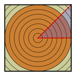
(image created in Lisp using Zach's Vecto library)How about two dimensions? This is immediately more awkward. The one-dimensional disk looks exactly like the one-dimensional square. In two dimensions, the disk and square are quite different. We either have to integrate over the square and calculate the radius of each point, or we have to integrate over increasing radii and be careful once we get to the in-radius of the square. (image created in Lisp using Zach's Vecto library)

I originally chose to try to integrate over the square. The probability density is \frac{1}{4} everywhere. This means the expected radius is \int_{y=-1}^1 \int_{x=-1}^1 \sqrt{x^2+y^2} dx dy. This gets to be no fun very fast since the inner integral comes out with a logarithm in it. I mean, do you want to finish this integral?

\int_{y=-1}^1 \left.\left( \frac{1}{2} x \sqrt{x^2 + y^2} + \frac{1}{2} y^2 \ln \left( x + \sqrt{x^2 + y^2} \right)\right)\right|_{x=-1}^1 dy

It may be easy. I didn’t want to mess with it. I suppose once you evaluate the x terms, it reduces a fair bit (if I did that all right):
\int_{y=-1}^1 \left( \sqrt{1 + y^2} + \frac{1}{2} y^2 \ln \left( \frac{1 + \sqrt{1 + y^2}}{-1 + \sqrt{1 + y^2}} \right) \right) dy

I still don’t want to touch it.

So, how about integrating over the radii? Again, the probability density is \frac{1}{4} everywhere. This makes the expected radius:

\int_{r=0}^1 \frac{1}{4} \cdot 2 \pi r dr + \int_{r=1}^{\sqrt{2}} \frac{1}{4} \cdot 8 \left( \frac{\pi}{4} - \arccos \frac{1}{r} \right) dr

With a little massaging, you can move the \frac{\pi}{4} from the second integral into the first instead:
\int_{r=0}^{\sqrt{2}} \frac{1}{4} \cdot 2 \pi r dr - \int_{r=1}^{\sqrt{2}} \frac{1}{4} \cdot 8 \arccos \frac{1}{r} dr

This is hardly consolation though. Here is where we get lost in our table of integrals for the better part of an hour.

And, this is only the two-dimensional case! In my original problem, the ambient space was 32-dimensional. My, oh my.

Updates In Email

Email:

l