Blur and Edge Detect your Fourier Transforms September 21st, 2009
Patrick Stein

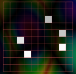
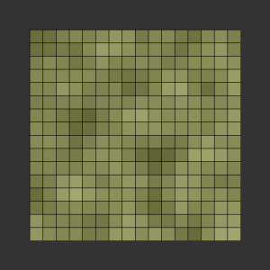
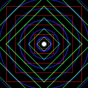
I have now added convolutions to my FFT Paint application. Here, I started with the following image (again, magnitude on the left and phase on the right):

conv_orig_m  conv_orig_p

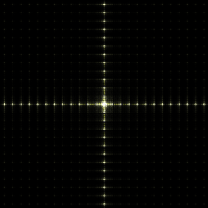
From there, I took the Fourier Transform:

conv_pre_m  conv_pre_p

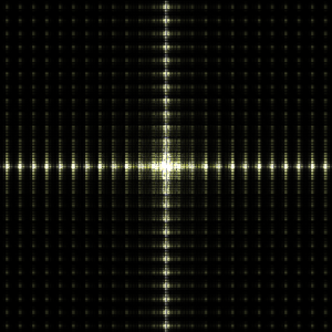
Then, I did a horizontal Sobel operator on it to get this:

conv_post_m  conv_post_p

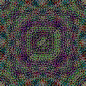
From there, I did the Inverse Fourier Transform to obtain this:

conv_final_m  conv_final_p

Enjoy!

Do Radial Gradients on your FFT September 16th, 2009
Patrick Stein

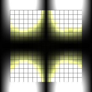
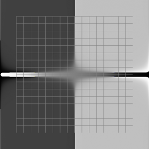
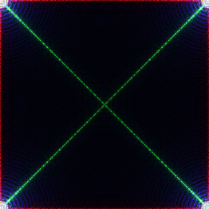
I have now added radial gradients to my FFT Paint application. Here, I wiped out an image entirely and painted my own data using only the new gradient tool to come up with this starting point:

mag_grad  phase_grad

This is what it looks like if I do the inverse FFT of that data. It’s not an incredibly interesting result, but it does show the power.

mag_inv  phase_inv

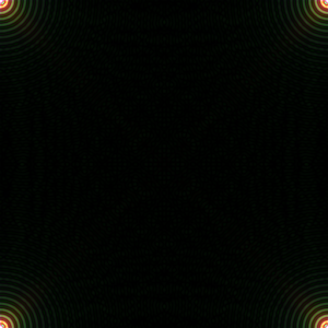
Here is another example of a starting point made entirely with the gradient paint tool:

conc_tm  conc_tp

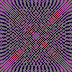
And, its resulting image when I do the inverse transform:

conc_rm  conc_rp

Simple Function Plotting in Javascript September 15th, 2009
Patrick Stein

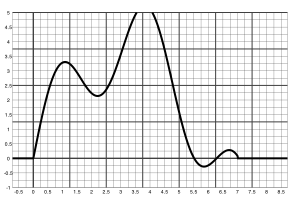
graphRather than work more on my FFT Paint program yesterday, I took a break to make a simple function plotter. There are lots of useful Java applets out there that do more than what I’ve done here. And, certainly, gnuplot is much more complete and useful.

On the other hand, if you just want to quickly plot something that you can save as an image, you either have to re-learn gnuplot (every time I use it, I have to sift through the help to figure out how to set up my tics and labels and output size and output filename) or you have to do screen grabs from one of the Java applets.

With the plotter that I wrote yesterday, you click on the Snapshot button, then right-click to save the image or copy it to your clipboard.

Enjoy.

Trapdoor Puzzles August 28th, 2009
Patrick Stein

With most logic or word puzzles, your goal is to find a solution. To make those puzzles interesting, the puzzle maker has to assure that there is a solution and that the solution is unique. This is true for crossword puzzles, sudoku puzzles, cryptograms, rebuses (rebi?), mazes, Lights Out games, and binary logic puzzles of this form: Alice is wearing red. John is older than Jimmy. The tallest person is not wearing green. Clue. Clue. Clue. Who is standing next to Alice? Rush Hour games and tanagrams are also usually crafted so that there is a unique solution.

Uniqueness

For some of these games, we mean a unique solution amongst all solutions without backtracking. For example, in solving a maze, we would not consider solutions that involve running down a corridor only to come back along the same corridor. For Lights Out games, the concept is simple but describing it takes work. Imagine that every square on the board, in addition to being lit or not, also has a letter ‘A’ on it at the start of the game. Whenever you press a button labelled ‘A’, it gets relabeled ‘B’. Every time you press a button labelled ‘B’, it gets relabeled ‘A’. Two solutions are identical if the board has the same configuration of ‘A’s and ‘B’s after both moves. Thus, hitting any button more than once was just a waste of time. However, the order that you hit the buttons makes no difference at all.

There is a notable crossword puzzle with two solutions. There are some notorious Sudoku puzzles with two solutions. I don’t know of any cryptograms with two solutions, but I am going to go asearchin’ some time.

Technically, a Sudoku puzzle with two solutions cannot be solved. You had to make a guess somewhere and it turned out you had twice the odds of being right that you should have. It is easy to accidentally take too many numbers out of the Sudoku grid and end up with an ambiguous puzzle. For a crossword puzzle, I doubt most people bother to check to see if the solution is unique. It probably is unique by sheer combinatorics. The same may be true cryptograms, as well. You’d have to specifically be trying to make them ambiguous to achieve it.

Trapdoors

Where are the trapdoors? Well, the puzzle creator has a much harder job than the puzzle solver for most games. It is easy to construct mazes and Lights Out games with unique solutions (in fact, it’s easy to show that if a Lights Out game is solvable, the solution is unique). It is not so easy to construct other puzzles that have provably unique solutions.

This brings us to the Discrete Logarithm Problem. Imagine that I told you that 3^x \equiv 16 \pmod{29} and asked you what x is modulo 28. There is no really easy way to solve this problem, yet it is easy to formulate such problems. I checked that 3^{14} \neq 1 \pmod{29}. Then, I picked x = 12 and plugged it in to see that 3^{12} \equiv 16 \pmod{29}. I started from the answer and was quickly able to generate a problem that I can guarantee has a unique solution.

This is called a trapdoor function. It is easy to calculate, but hard to invert the calculation. It’s also not a very fun problem to do. You will never open up the comics page of your newspaper and find five of these problems below the bridge column and above the horoscopes.

I can easily imagine a whole variety of Lights Out type games where lights have more than one state. It would be easy to prove, for a wide class of such games, that when a solution exists, it is unique. These would all be solvable by inverting a matrix whose coefficients come from a finite field.

What other puzzles could take advantage of trapdoor functions to make the game easier on the puzzle maker than on the puzzle solver?
Taking the Long Way Home August 14th, 2009
Patrick Stein

I was pondering non-deterministic, shareware nagging. Suppose that every time you performed a particular function, I wanted to randomly decide whether to nag you this time or not. Suppose further that I’d prefer not to have to keep track of how long it’s been since I last nagged you, but I’d still like you to be nagged about once every n times. Naïvely, one would expect that if I just chose a random number uniformly from the range zero to one and nag if the number is less than \frac{1}{n}, this would do the trick. You would expect that if you rolled an n-sided die each time, that you’d roll a one about every n-th time.

Me, I’ve learned to never trust my naïve intuition when it comes to probability questions. Well, it turns out that the naïve answer is perfectly correct in this case. Here is the epic journey I took to get there though.

Here’s what I wanted. I wanted to know the probability p needed so the expected number of trials until the first success is some number n given that each trial is independent and is successful p proportion of the time. Suppose for a moment that I decided I am going to roll a six-sided die until I get a one. What is the expected number of times that I need to roll that die to get my first one? What I want here is the inverse problem. How many sides should my die be if I want it to take n tries (on average) to get my first one?

tree In the picture at the right, each circle represents a trial. Each square represents a success. What I am looking for is what value should I pick for p so that if you go left p proportion of the time and go right the other (1-p) proportion of the time, you will expect to hit n circles along your descent. You could, if very unlucky (or lucky in this case since I’m going to nag you) go forever to the right and never get to a rectangle. So, already, we’re expecting an infinite sum.

Indeed, the expected number of circles you cross in a random descent of this tree is E(p) = \sum_{k=1}^{\infty} k \cdot p \cdot (1 - p)^{k-1}. Massaging this a little, we can get it into a simpler form: E(p) = \frac{p}{1-p} \sum_{k=1}^{\infty} k \cdot (1 - p)^k.

That infinite series is pretty nasty looking though. So, we whip out a handy table of infinite series and see that:

\sum_{k=1}^{\infty} k^m q^k = \frac{1}{(1-q)^{m+1}} \sum_{k=0}^m \left[ \sum_{j=0}^{k+1} (-1)^j { {m+1} \choose j } (k - j + 1)^m \right] q^{m-k}

Fortunately, in our case, m = 1. As such, we can reduce this significantly:
\frac{1}{(1-q)^2} \sum_{k=0}^1 \left[ \sum_{j=0}^{k+1} (-1)^j { 2 \choose j } (k - j + 1) \right] q^{1-k}

\frac{1}{(1-q)^2} \left\{ \left[ \sum_{j=0}^1 (-1)^j { 2 \choose j } (1 - j) \right] q + \left[ \sum_{j=0}^2 (-1)^j { 2 \choose j } (2 - j) \right] \right\}

Now, we note that when j = 2, the last summand is zero. So, \sum_{j=0}^2 (-1)^j { 2 \choose j } (2 - j) = \sum_{j=0}^1 (-1)^j {2 \choose j } (2 - j). As such, we can combine our two summations into one:
\frac{1}{(1-q)^2} \sum_{j=0}^1 (-1)^j { 2 \choose j } \left[ (1 - j) q + (2 - j) \right]

And, since j is only going from zero to one, it’s easy enough to write out both terms of the summation:
\frac{1}{(1-q)^2} \left\{ { 2 \choose 0 } \left[ q + 2 \right] - { 2 \choose 1 } \right\}

\frac{1}{(1-q)^2} \left\{ q + 2 - 2 \right\}

\sum_{k=1}^{\infty} k q^k = \frac{q}{(1-q)^2}

Whew! Big sigh. We’re through the ugly parts. Now, in our case, q = (1-p), and the equation we were interested in was E(p) = \frac{p}{1-p} \sum_{k=1}^{\infty} k \cdot (1 - p)^k. Plugging in (1-p) for the q in our infinite series solution, we find that

E(p) = \frac{p}{1-p} \cdot \frac{1-p}{p^2} = \frac{1}{p}

Two pages of ugly, ugly algebra bears out the simple guess. Wheee! If we want E(p) = n, then we have to pick p = \frac{1}{n}. Hooray!

Updates In Email

Email:

l