Math :: nklein software

Lines Are Big Circles September 13th, 2013
Patrick Stein

In previous posts here, I described using Clifford algebras for representing points and rotations. I was never very satisfied with this because the translations were still tacked on rather than incorporated in the algebra. To represent geometric objects, you need to track two Clifford multivectors: one for the orientation and another for the offset.

About two weeks ago, I found David Hestenes’s paper Old Wine in New Bottles: A new algebraic framework for computational geometry. In that paper, he describes a way to use Clifford Algebras to unify the representation of points, lines, planes, hyperplanes, circles, spheres, hyperspheres, etc. This was a big bonus. By using a projective basis, we can unify the orientation and offset. By using a null basis, we can bring in lines, planes, hyperplanes, circles, spheres, and hyperspheres.

The null basis ends up giving you a point at infinity. Every line goes through the point at infinity. None of the circles do. But, if you think of a line as a really, really big circle that goes through infinity, now you have unified lines and circles. Circles and lines are both defined by three points in the plane. (Technically, you can define a line with any three collinear points, but then you need to craft a point collinear to the other two. The point at infinity is collinear with every line. Further, such things could be seen as flattened circles having finite extent (diameter equal to the distance between the furthest apart of the three points) rather than an infinite line.)

So, I need to use Clifford algebras with a projective and null basis. All of the playing I previously did with Clifford algebras was using an orthonormal basis.

What is a basis?

To make a Clifford algebra, one starts with a vector space. A vector space has a field of scalars (real numbers, usually) and vectors. You can multiply any vector by a scalar to get another vector. And, if $\alpha$ and $\beta$ are scalars and $\textbf{v}$ is a vector, then $\alpha (\beta \textbf{v}) = (\alpha \beta)\textbf{v}$ . And, of course, we want $1\textbf{v} = \textbf{v}$ (in fact, even if $1\textbf{v}$ weren’t $\textbf{v}$ exactly, we’re always going to be multiplying by at least $1$ , so we can recast our thinking to think about $1\textbf{v}$ any place we write $\textbf{v}$ ).

You can add together any two vectors to get another vector. Further, this addition is completely compatible with the scalar multiplication so that $\alpha\textbf{v} + \beta\textbf{v} = (\alpha + \beta)\textbf{v}$ and $\alpha(\textbf{v} + \textbf{w}) = \alpha\textbf{v} + \alpha\textbf{w}$ . This of course means that every vector has a negative vector. Further $0\textbf{v} = 0\textbf{w}$ for all vectors $\textbf{v}$ and $\textbf{w}$ . This is the distinguished vector called the zero vector. The sum of any vector $\textbf{v}$ and the zero vector is just the vector $\textbf{v}$ .

Every vector space has a basis (though some have an infinite basis). A basis is a minimal subset of the vectors such that every vector vector can be written as the sum of multiples of the basis vectors. So, if the whole basis is $\textbf{v}$ and $\textbf{w}$ , then every vector can be written as $\alpha\textbf{v} + \beta\textbf{w}$ . A basis is a minimal subset in that no basis element can be written as the sum of multiples of the other elements. Equivalently, this means that the only way to express the zero vector with the basis is by having every basis element multiplied by the scalar zero.

Okay, but what is an orthonormal basis?

You need more than just a vector space to make a Clifford algebra. You need either a quadratic form or a dot-product defined on the vectors.

A quadratic form on a vector is a function $Q$ that takes in a vector and outputs a scalar. Further, $Q(\alpha\textbf{v}) = \alpha^2 Q(\textbf{v})$ for all scalars $\alpha$ and all vectors $\textbf{v}$ .

A dot product is a function $\langle\cdot{},\cdot{}\rangle$ that takes two vectors and outputs a scalar. A dot product must be symmetric so that $\langle\textbf{v},\textbf{w}\rangle = \langle\textbf{w},\textbf{v}\rangle$ for all vectors $\textbf{v}$ and $\textbf{w}$ . Furthermore, the dot product must be linear in either term. (Since it’s symmetric, it suffices to require it be linear in either term.) This means that for all scalars $\alpha$ and $\beta$ and all vectors $\textbf{v}$ , $\textbf{w}$ , and $\textbf{x}$ then $\langle\alpha\textbf{v}+\beta\textbf{w},\textbf{x}\rangle = \alpha\langle\textbf{v},\textbf{x}\rangle + \beta\langle\textbf{w},\textbf{x}\rangle$ .

From any dot product, you can make a quadratic form by saying $Q(\textbf{x}) = \langle\textbf{x},\textbf{x}\rangle$ $\textbf{}$ . And, so long as you’re working with scalars where one can divide by two (aka, almost always), you can make a dot product from a quadratic form by saying $\langle\textbf{x},\textbf{y}\rangle = \frac{1}{2}(Q(\textbf{x}+\textbf{y}) - Q(\textbf{x}) - Q(\textbf{y})$ . So, it doesn’t really matter which you have. I’m going to freely switch back and forth between them here for whichever is most convenient for the task at hand. I’ll assume that I have both.

So, let’s say we have a dot product on our vector space. What happens when we take the dot product on pairs of our basis vectors? If $\textbf{v}$ and $\textbf{w}$ are distinct elements of our basis with $\langle\textbf{v},\textbf{w}\rangle = 0$ $\textbf{}$ , then $\textbf{v}$ and $\textbf{w}$ are said to be orthogonal (basis elements). If every element of the basis is orthogonal to every other basis element, then we have an orthogonal basis.

We say a basis element $\textbf{v}$ is normalized if $\langle\textbf{v},\textbf{v}\rangle = \pm 1$ . If all of the basis vectors are normalized, we have a normal basis.

An orthonormal basis is a basis that’s both an orthogonal basis and a normal basis.

You can represent any dot product as a symmetric matrix $A$ . To find $\langle\textbf{v},\textbf{w}\rangle$ , you multiply $\textbf{v}^TA\textbf{w}$ . Further, you can always decompose a scalar matrix into the form $A = S D S^T$ where $D$ is a diagonal matrix (a matrix where all of the elements off of the diagonal are zero) and $S^T = S^{-1}$ . Because of that, you can always find an orthogonal basis for a vector space. So, with just a little bit of rotating around your original choice of basis set, you can come up with a different basis that is orthogonal.

If your orthogonal basis is not normalized, you can (almost always) normalize the basis vectors where $Q(\textbf{v}) \ne 0$ by dividing it by the square root of $Q(\textbf{v})$ . If any of the elements on the diagonal in the diagonal matrix are zero, then you didn’t have a minimal set for a basis.

So, as long as you can divide by square roots in whatever numbers system you chose for your scalars, then you can find an orthonormal basis. That means that $Q(\textbf{v})$ is either $+1$ or $-1$ for every basis vector $\textbf{v}$ . It also means (going back to dot product) that $\langle\textbf{v},\textbf{w}\rangle = 0$ for distinct basis vectors $\textbf{v}$ and $\textbf{w}$ .

You can also re-order your basis set so that all of the $Q(\textbf{v}) = +1$ vectors come first and all of the $Q(\textbf{v}) = -1$ vectors are last. So, much of the literature on Clifford algebras (and all of the stuff that I had done before with them) uses such a basis. If the field of scalars is the real numbers $\mathbb{R}$ , then we abbreviate the Clifford algebra as $\mathcal{C}\ell_{p,q}$ when there are $p$ basis vectors where $Q(\textbf{v}) = +1$ and $q$ basis vectors where $Q(\textbf{v}) = -1$ .

What about Projective and Null?

I mentioned at the outset that the Hestenes paper uses a projective basis that’s also a null basis. If you’ve done any geometry in computers before you have probably bumped into projective coordinates. If you have a 3d-vector $[x,y,z]^T$ then you turn it into a projective coordinate by making it a 4d-vector that ends with $1$ giving you $[x,y,z,1]^T$ . Now, you take your three by three rotation matrices and extend them to four by four matrices. This lets you incorporate rotations and translations into the same matrix instead of having to track a rotation and an offset.

What about a null basis though? With a null basis, $Q(\textbf{v}) = 0$ for each (some?) of the basis vectors. The key point for me here is that the matrix representing the dot product isn’t diagonal. As an easy example, if we have a basis with two basis vectors $\textbf{v}$ and $\textbf{w}$ , then we can represent any vector $\textbf{x}$ as $\alpha\textbf{v} + \beta\textbf{w}$ . If we have $Q(x) = \alpha^2 - \beta^2$ , then that is an orthonormal basis (with $Q(\textbf{v}) = +1$ and $Q(\textbf{w}) = -1$ ). If we picked two different basis vectors $\textbf{v}^\prime$ and $\textbf{w}^\prime$ then we would represent $\textbf{x}$ as $\alpha^\prime\textbf{v}^\prime + \beta^\prime\textbf{w}^\prime$ . We could pick them so that $Q(\textbf{x}) = 2\alpha^\prime\beta^\prime$ . This would be a null basis because $Q(\textbf{v}^\prime) = Q(\textbf{w}^\prime) = 0$ .

Clifford Algebras with an Orthonormal Basis

Once you have a vector space and a quadratic form or dot product, then you make a Clifford algebra by defining a way to multiply vectors together. For Clifford algebras, we insist that when we multiply a vector $\textbf{v}$ by itself, the result is exactly $Q(\textbf{v})$ . Then, we go about building the biggest algebra we can with this restriction.

Let’s look at what happens when we have two vectors $\textbf{v}$ and $\textbf{w}$ . Our Clifford restriction means that $(\textbf{v}+\textbf{w})^2 = Q(\textbf{v}+\textbf{w})$ . We want multiplication to distribute with addition just like it does in algebra so the left hand side there should be: $\textbf{v}^2 + \textbf{vw} + \textbf{wv} + \textbf{w}^2$ . Note: we haven’t yet assumed that our multiplication has to be commutative, so we can’t reduce that to $\textbf{v}^2 + 2 \textbf{vw} + \textbf{w}^2$ .

Remember, now, the connection between the quadratic form $Q$ and the dot product $\langle\cdot,\cdot\rangle$ . We have, for the right hand side, that $Q(\textbf{v}+\textbf{w}) = \langle\textbf{v}+\textbf{w},\textbf{v}+\textbf{w}\rangle$ . Now, we use the fact that the dot product is linear in both terms to say that $\langle\textbf{v}+\textbf{w},\textbf{v}+\textbf{w}\rangle = \langle\textbf{v},\textbf{v}\rangle + \langle\textbf{v},\textbf{w}\rangle + \langle\textbf{w},\textbf{v}\rangle + \langle\textbf{w},\textbf{w}\rangle$ . Using the connection to the quadratic form again and the fact that the dot product is symmetric, we can simplify that to $Q(\textbf{v}) + 2\langle\textbf{v},\textbf{w}\rangle + Q(\textbf{w})$ .

Because $v^2 = Q(\textbf{v})$ and $w^2 = Q(\textbf{w})$ , we can simplify our original equation $(\textbf{v}+\textbf{w})^2 = Q(\textbf{v}+\textbf{w})$ to be $\textbf{vw} + \textbf{wv} = 2\langle\textbf{v},\textbf{w}\rangle$ .

If $\textbf{v} = \textbf{w}$ , then the above reduces to the definitional $\textbf{v}^2 = Q(v)$ . If $\textbf{v}$ and $\textbf{w}$ are distinct basis vectors in our orthogonal basis, then $2\langle\textbf{v},\textbf{w}\rangle = 0$ . This means that $\textbf{wv} = -\textbf{vw}$ . So, our multiplication of distinct basis vectors anticommutes!

Now, given an arbitrary vector, we can express it as a sum of multiples of the basis vectors: $\textbf{v} = \alpha_1\textbf{e}_1 + \alpha_2\textbf{e}_2 + ...$ where the $\alpha_i$ are all scalars and the $\textbf{e}_i$ are all basis vectors in our orthogonal basis. Given two such vectors we can do all of the usual algebraic expansion to express the product of the two vectors as a sum of multiples of products of pairs of basis vectors. Any place where we end up with $\textbf{e}_i\textbf{e}_i$ we can replace it with the scalar number $Q(\textbf{e}_i)$ . Any place we end up with $\textbf{e}_i\textbf{e}_j$ with $i < j$ , we can leave it as it is. Any place we end up with $\textbf{e}_j\textbf{e}_i$ with $i < j$ , we can replace it with $-\textbf{e}_i\textbf{e}_j$ . Then, we can gather up like terms.

So, suppose there were two vectors in our orthonormal basis $\textbf{e}_1$ and $\textbf{e}_2$ . And, assume $Q(\textbf{e}_1) = +1$ and $Q(\textbf{e}_2) = -1$ . Then $(a\textbf{e}_1 + b\textbf{e}_2)(c\textbf{e}_1 + d\textbf{e}_2)$ expands out to $ac\textbf{e}_1^2 + ad\textbf{e}_1\textbf{e}_2 + bc\textbf{e}_2\textbf{e}_1 + bd\textbf{e}_2^2$ . We can then manipulate that as outlined in the previous paragraph to whittle it down to $(ac-bd) + (ad-bc)\textbf{e}_1\textbf{e}_2$ .

We still don’t know what $\textbf{e}_1\textbf{e}_2$ is exactly, but we’re building a big-tent algebra here. We don’t have a restriction that says it has to be something, so it gets to be its own thing unless our restrictions hold it back. How big is our tent going to be? Well, let’s see what happens if we multiply $\textbf{e}_1\textbf{e}_2$ by other things we already know about.

What happens if we multiply $\textbf{e}_1(\textbf{e}_1\textbf{e}_2)$ ? We want our multiplication to be associative. So, $\textbf{e}_1(\textbf{e}_1\textbf{e}_2) = \textbf{e}_1^2\textbf{e}_2$ and because $\textbf{e}_1^2 = 1$ , this is just $\textbf{e}_1(\textbf{e}_1\textbf{e}_2) = \textbf{e}_2$ . Well, what if we had multiplied in the other order? $(\textbf{e}_1\textbf{e}_2)\textbf{e}_1 = -(\textbf{e}_2\textbf{e}_1)\textbf{e}_1 = -\textbf{e}_2\textbf{e}_1^2 = -\textbf{e}_2$ . Interesting. By similar reasoning, $\textbf{e}_2(\textbf{e}_1\textbf{e}_2) = -\textbf{e}_2^2\textbf{e}_1 = \textbf{e}_1$ and $(\textbf{e}_1\textbf{e}_2)\textbf{e}_2 = \textbf{e}_1\textbf{e}_2^2 = -\textbf{e}_1$ .

What happens if we multiply $(\textbf{e}_1\textbf{e}_2)(\textbf{e}_1\textbf{e}_2)$ . This is just a combination of the above sorts of things and we find that

$(\textbf{e}_1\textbf{e}_2)^2 = -(\textbf{e}_2\textbf{e}_1)(\textbf{e}_1\textbf{e}_2) = -\textbf{e}_2(\textbf{e}_1^2)\textbf{e}_2 = -\textbf{e}_2^2 = 1$

So, that’s as big as our tent is going to get with only two vectors in our orthonormal basis.

Our Clifford algebra then has elements composed of some multiple of the scalar $1$ plus some multiple of $\textbf{e}_1$ plus some multiple of $\textbf{e}_2$ plus some multiple of $\textbf{e}_1\textbf{e}_2$ . If we had added a third basis vector $\textbf{e}_3$ , then we also get $\textbf{e}_1\textbf{e}_3$ , $\textbf{e}_2\textbf{e}_3$ , and $\textbf{e}_1\textbf{e}_2\textbf{e}_3$ . In general, if you have $n$ vectors in the basis of the vector space, then there will be $2^n$ basis elements in the corresponding Clifford algebra.

You can rework any term $\alpha\textbf{e}_i\textbf{e}_j\textbf{e}_k...$ so that the subscripts of the basis vectors are monotonically increasing by swapping adjacent basis vectors with differing subscripts changing the sign on $\alpha$ at the same time. When you have two $\textbf{e}_i$ side-by-side with the same subscript, annihilate them and multiply the coefficient $\alpha$ by $Q(e_i)$ (which was either $+1$ or $-1$ ). Then, you have a reduced term $\pm\alpha\textbf{e}_i\textbf{e}_j...$ where the subscripts are strictly increasing.

What Happens When You Don’t Have An Orthonormal Basis?

The Hestenes paper doesn’t use an orthonormal basis. I’d never played with Clifford algebras outside of one. It took me about two weeks of scrounging through text books and information about something called the contraction product and the definitions of Clifford algebras in terms of dot-products plus something called the outer product (which gives geometric meaning to our new things like $\textbf{e}_1\textbf{e}_2$ ).

I learned a great deal about how to multiply vectors, but I didn’t feel that much closer to being able to multiply $\textbf{e}_1\textbf{e}_4\textbf{e}_3\textbf{e}_1$ unless the basis was orthonormal. I felt like I’d have to know things like the dot product of a vector with something like $\textbf{e}_4\textbf{e}_3\textbf{e}_1$ and then somehow mystically mix in the contraction product and extend by linearity.

There’s a whole lot of extending by linearity in math. In some cases, I feel like extending by linearity leaves me running in circles. (To go with the theme, sometimes I’m even running in a really big circle through the point at infinity.) We did a bit of extending by linearity above when we went from $\textbf{v}^2 = Q(\textbf{v})$ into what $(\textbf{v}+\textbf{w})^2$ must be based on the linearity in the dot product.

Finally, something clicked for me enough to figure out how to multiply $\textbf{e}_1\textbf{e}_4\textbf{e}_3\textbf{e}_1$ and express it as a sum of terms in which the basis vectors in each term had increasing subscripts. Now that it has clicked, I see how I should have gone back to one of our very first equations: $\textbf{vw} + \textbf{wv} = 2\langle\textbf{v},\textbf{w}\rangle$ . With our orthogonal basis, $\langle\textbf{v},\textbf{w}\rangle$ was always zero for distinct basis vectors.

If we don’t have an orthogonal basis, then the best we can do is $\textbf{wv} = 2\langle\textbf{v},\textbf{w}\rangle - \textbf{vw}$ . That is good enough. Suppose then we want to figure out $\textbf{e}_1\textbf{e}_4\textbf{e}_3\textbf{e}_1$ so that none of the terms have subscripts out of order. For brevity, let me write $d_{i,j}$ to mean $\langle\textbf{e}_i,\textbf{e}_j\rangle$ . The first things we see out of order are $\textbf{e}_4$ and $\textbf{e}_3$ . To swap those, we have to replace $\textbf{e}_4\textbf{e}_3$ with $d_{3,4} - \textbf{e}_3\textbf{e}_4$ . Now, we have $\textbf{e}_1 ( 2d_{3,4} - \textbf{e}_3\textbf{e}_4 ) \textbf{e}_1$ . With a little bit of algebra, this becomes $2d_{3,4}\textbf{e}_1^2 - \textbf{e}_1\textbf{e}_3\textbf{e}_4\textbf{e}_1 = 2d_{3,4}d_{1,1} - \textbf{e}_1\textbf{e}_3\textbf{e}_4\textbf{e}_1$ . That last term is still not in order, so we still have more to do.

$\begin{array}{c}2d_{3,4}d_{1,1} - \textbf{e}_1\textbf{e}_3\textbf{e}_4\textbf{e}_1 \\2d_{3,4}d_{1,1} - \textbf{e}_1\textbf{e}_3(2d_{1,4} - \textbf{e}_1\textbf{e}_4) \\2d_{3,4}d_{1,1} - 2d_{1,4}\textbf{e}_1\textbf{e}_3 + \textbf{e}_1\textbf{e}_3\textbf{e}_1\textbf{e}_4 \\2d_{3,4}d_{1,1} - 2d_{1,4}\textbf{e}_1\textbf{e}_3 + \textbf{e}_1(2d_{1,3} - \textbf{e}_1\textbf{e}_3)\textbf{e}_4 \\2d_{3,4}d_{1,1} - 2d_{1,4}\textbf{e}_1\textbf{e}_3 + 2d_{1,3}\textbf{e}_1\textbf{e}_4 - \textbf{e}_1^2\textbf{e}_3\textbf{e}_4 \\2d_{3,4}d_{1,1} - 2d_{1,4}\textbf{e}_1\textbf{e}_3 + 2d_{1,3}\textbf{e}_1\textbf{e}_4 - d_{1,1}\textbf{e}_3\textbf{e}_4\end{array}$

Whew. Now, to get that into code.

26 SLOC

In the end, I ended up with this 26 SLOC function that takes in a matrix dots to represent the dot product and some number of ordered lists of subscripts and returns a list of scalars where the scalar in spot $i$ represents the coefficient in front of the ordered term where the $k$ -th basis vector is involved if the $(k-1)$ -th bit of $i$ is set. So, for the example we just did with the call (basis-multiply dots '(1 4) '(3) '(1)), the zeroth term in the result would be $2d_{3,4}d_{1,1}$ . The fifth term ( $(2^2 + 2^0)$ -th term) would be $-2d_{1,4}$ . The ninth term would be $2d_{1,3}$ . The twelfth term would be $-d{1,1}$ . The rest of the terms would be zero.

From this, I will be able to build a function that multiplies arbitrary elements of the Clifford algebra. Getting to this point was the hard part for me. It is 26 SLOC that took me several weeks of study to figure out how to do on paper and about six hours of thinking to figure out how to do in code.

(defun basis-multiply (dots &rest xs)
(let ((len (expt 2 (array-dimension dots 0))))
(labels ((mul (&rest xs)
(let ((xs (combine-adjacent (remove nil xs))))
(cond
((null xs)
(vec len 0))

((null (rest xs))
(vec len (from-bits (first xs))))

(t
(destructuring-bind (x y . xs) xs
(let ((a (first (last x)))
(b (first y))
(x (butlast x))
(y (rest y)))
(if (= a b)
(combine-like x a y xs)
(swap-ab x a b y xs))))))))

(dot (a b)
(aref dots (1- a) (1- b)))

(combine-like (x a y xs)
;; X e1 e1 Y ... = (e1.e1) X Y ...
(vs (dot a a) (apply #'mul x y xs)))

(swap-ab (x a b y xs)
;; X e2 e1 Y ... = 2(e1.e2) X Y ... - X e1 e2 Y ...
(v- (vs (* 2 (dot a b)) (apply #'mul x xs))
(apply #'mul x (list b a) y xs))))
(apply #'mul xs))))

I had one false start on the above code where I accidentally confounded the lists that I was using as input with the lists that I was generating as output. I had to step back and get my code to push all of the work down the call stack while rolling out the recursion and only creating new vectors during the base cases of the recursion and only doing vector subtractions while unrolling the recursion.

There are also 31 SLOC involved in the combine-adjacent function (which takes a list like ((1 2 3) nil (4 5) (3)) and removes the nils then concatenates consecutive parts that are in order already to get ((1 2 3 4 5) (3))), the vec function (which makes a vector of a given length with a non-zero coefficient in a given location), the from-bits function (which turns a list of integers into a number with the bit $k$ set if $k+1$ is in the list) and the little functions like vs and v- (which, respectively, scale a list of numbers by a factor and element-wise subtract two lists).

The 31 supporting SLOC were easy though. The 26 SLOC shown above represent the largest thought-to-code ratio of any code that I’ve ever written.

WO0T!!!t!1! or something!

Now, to Zig this SLOC for Great Justice!

Visualizing Galois Fields (Follow-up) May 21st, 2012
Patrick Stein

In my previous article, I should have finished by remapping the multiplication and addition tables so that the multiplication table was in cyclic order. In cyclic order, the zeroth column (or row) represents zero and the $(i+1)$ -th column (or row) (for $i \neq 0$ ) represents $a^i$ for some generator $a$ . As such, the multiplication table is simply $0$ in the zeroth row and column and $1 + ((i+j) \mod 255)$ for the spot $(i+1,j+1)$ .

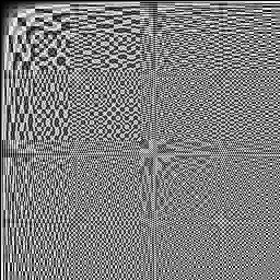
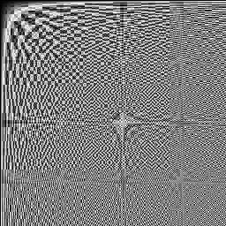
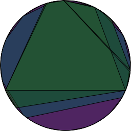
Once resorted by the order of the powers of a generator $a$ , the multiplication table look the same regardless of the $a$ . The addition, however, looks different for different generators. Below are the addition tables for two of them: $a = (1+x)$ on the right and $a = x^3 + x^6 + x^7$ on the left. They make as decent a stereo as any of the other pairs so far.

Here’s the code that I used to generate the remapping for a given generator.

(defun make-cyclic-remapping (fn generator &optional (limit 256))
(let ((to (make-array (list limit) :initial-element 0))
(from (make-array (list limit) :initial-element 0))
(used (make-hash-table :test #'equal)))
;; fill up the lookup tables
(setf (gethash 0 used) t)
(nlet fill-tables ((exp 1) (acc 1))
(when (< exp limit)
(setf (aref to exp) acc
(aref from acc) exp
(gethash acc used) t)
(fill-tables (1+ exp) (funcall fn acc generator))))
;; return a closure around the lookup tables
(when (= (hash-table-count used) limit)
(lambda (direction n)
(ecase direction
(:to (aref to n))
(:from (aref from n)))))))

If you’ve read it, you can probably tell by my code that I’m still under the influence of Let Over Lambda. If you haven’t read it, it is quite worth the read.

Then, I used a modified version of the draw-heightmap function which also takes in the remapping function.

(defun draw-mapped-heightmap (op map filename &optional (limit 256))
(let ((png (make-instance 'zpng:pixel-streamed-png
:color-type :grayscale
:width limit
:height limit)))
(with-open-file (stream filename
:direction :output
:if-does-not-exist :create
:element-type '(unsigned-byte 8))
(zpng:start-png png stream)
(dotimes (xx limit)
(dotimes (yy limit)
(let* ((a (funcall map :to xx))
(b (funcall map :to yy))
(c (funcall map :from (funcall op a b))))
(zpng:write-pixel (list c) png))))
(zpng:finish-png png)))
(values))

Visualizing Galois Fields May 17th, 2012
Patrick Stein

Galois fields are used in a number of different ways. For example, the AES encryption standard uses them.

Arithmetic in Galois Fields

The Galois fields of size $2^n$ for various $n$ are convenient in computer applications because of how nicely they fit into bytes or words on the machine. The Galois field $GF(2^n)$ has $2^n$ elements. These elements are represented as polynomials of degree less than $n$ with all coefficients either 0 or 1. So, to encode an element of $GF(2^n)$ as a number, you need an $n$ -bit binary number.

For example, let us consider the Galois field $GF(2^3)$ . It has $2^3 = 8$ elements. They are (as binary integers) $000$ , $001$ , $010$ , $011$ , $100$ , $101$ , $110$ , and $111$ . The element $110$ , for example, stands for the polynomial $x^2 + x$ . The element $011$ stands for the polynomial $x + 1$ .

The coefficients add together just like the integers-modulo-2 add. In group theory terms, the coefficients are from $\mathbb{Z}/2\mathbb{Z}$ . That means that $0 + 0 = 0$ , $0 + 1 = 1$ , $1 + 0 = 1$ , and $1 + 1 = 0$ . In computer terms, $a + b$ is simply $a$ XOR $b$ . That means, to get the integer representation of the sum of two elements, we simply have to do the bitwise-XOR of their integer representations. Every processor that I’ve ever seen has built-in instructions to do this. Most computer languages support bitwise-XOR operations. In Lisp, the bitwise-XOR of $a$ and $b$ is (logxor a b).

Multiplication is somewhat trickier. Here, we have to multiply the polynomials together. For example, $(x + 1) \cdot x = x^2 + x$ . But, if we did $(x^2 + x) \cdot x$ , we’d end up with $x^3 + x^2$ . We wanted everything to be polynomials of degree less than $n$ and our $n$ is 3. So, what do we do?

What we do, is we take some polynomial of degree $n$ that cannot be written as the product of two polynomials of less than degree $n$ . For our example, let’s use $x^3 + x + 1$ (which is $1011$ in our binary scheme). Now, we need to take our products modulo this polynomial.

You may not have divided polynomials by other polynomials before. It’s a perfectly possible thing to do. When we divide a positive integer $a$ by another positive integer $b$ (with $b$ bigger than 1), we get some answer strictly smaller than $a$ with a remainder strictly smaller than $b$ . When we divide a polynomial of degree $m$ by a polynomial of degree $n$ (with $n$ greater than zero), we get an answer that is a polynomial of degree strictly less than $m$ and a remainder that is a polynomial of degree strictly less than $n$ .

Dividing proceeds much as long division of integers does. For example, if we take the polynomial (with integer coefficients) $x^3 + 2x + 5$ and divide it by the polynomial $x + 3$ , we start by writing it as:

$x + 3 \overline{\left) x^3 + 0x^2 + 2x + 5\right.}$ We notice that to get $(x+3) \cdot q(x)$ to start with $x^3$ , we need $q(x)$ to start with $x^2$ . We then proceed to subtract $(x+3) \cdot x^2$ and then figure out that we need a $-3x$ for the next term, and so on. We end up with $x^2 - 3x + 11$ with a remainder of $-28$ (a degree zero polynomial).

$\begin{array}{ccrcrcrcr}& & & & x^2 & - & 3x & + & 11 \\& \multicolumn{8}{l}{\hrulefill} \\(x+3) & ) & x^3 & + & 0x^2 & + & 2x & + & 5 \\& & x^3 & + & 3x^2 & & & & \\& & \multicolumn{3}{l}{\hrulefill} & & & & \\& & & - & 3x^2 & + & 2x & & \\& & & - & 3x^2 & - & 9x & & \\& & & \multicolumn{4}{l}{\hrulefill} & & \\& & & & & & 11x & + & 5 \\& & & & & & 11x & + & 33 \\& & & & & & \multicolumn{3}{l}{\hrulefill} \\& & & & & & & - & 28\end{array}$ For the example we cited earlier we had $x^3 + x^2$ which we needed to take modulo $x^3 + x + 1$ . Well, dividing $x^3 + x^2$ by $x^3 + x + 1$ , we see that it goes in one time with a remainder of $x^2 + x + 1$ . [Note: addition and subtraction are the same in $GF(2^n)$ .]

$\begin{array}{ccrcrcrcr}& & & & & & & & 1 \\& \multicolumn{8}{l}{\hrulefill} \\(x^3+x+1) & ) & x^3 & + & x^2 & + & 0x & + & 0 \\& & x^3 & + & 0x^2 & + & x & + & 1 \\& & \multicolumn{7}{l}{\hrulefill} \\& & & & x^2 & + & x & + & 1\\\end{array}$ For a reasonable way to accomplish this in the special case of our integer representations of polynomials in $GF(2^n)$ , see this article about Finite Field Arithmetic and Reed Solomon Codes. In (tail-call style) Lisp, that algorithm for $GF(2^8)$ might look something like this to multiply $a$ times $b$ modulo $m$ :

(flet ((next-a (a)
(ash a -1))
(next-b (b)
(let ((overflow (plusp (logand b #x80))))
(if overflow
(mod (logxor (ash b 1) m) #x100)
(ash b 1)))))
(labels ((mult (a b r)
(cond
((zerop a) r)
((oddp a) (mult (next-a a) (next-b b) (logxor r b)))
(t (mult (next-a a) (next-b b) r)))))
(mult a b 0)))

How is the Galois field structured?

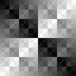
The additive structure is simple. Using our 8-bit representations of elements of $GF(2^8)$ , we can create an image where the pixel in the $i$ -th row and $j$ -th column is the sum (in the Galois field) of $i$ and $j$ (written as binary numbers). That looks like this:

Just before the above-mentioned article hit reddit, I got to wondering if the structure of the Galois field was affected at all by the choice of polynomial you used as the modulus. So, I put together some code to try out all of the polynomials of order 8.

Remember way back at the beginning of multiplication, I said that the modulus polynomial had to be one which couldn’t be written as the product of two polynomials of smaller degree? If you allow that, then you have two non-zero polynomials that when multiplied together will equal your modulus polynomial. Just like with integers, if you’ve got an exact multiple of the modulus, the remainder is zero. We don’t want to be able to multiply together two non-zero elements to get zero. Such elements would be called zero divisors.

Zero divisors would make these just be Galois rings instead of Galois fields. Another way of saying this is that in a field, the non-zero elements form a group under multiplication. If they don’t, but multiplication is still associative and distributes over addition, we call it a ring instead of a field.

Galois rings might be interesting in their own right, but they’re not good for AES-type encryption. In AES-type encryption, we’re trying to mix around the bits of the message. If our mixing takes us to zero, we can never undo that mixing—there is nothing we can multiply or divide by to get back what we mixed in.

So, we need a polynomial that cannot be factored into two smaller polynomials. Such a polynomial is said to be irreducible. We can just start building an image for the multiplication for a given modulus and bail out if it has two non-zero elements that multiply together to get zero. So, I did this for all elements which when written in our binary notation form odd numbers between (and including) 100000001 and 111111111 (shown as binary). These are the only numbers which could possibly represent irreducible polynomials of degree 8. The even numbers are easy to throw out because they can be written as $x$ times a degree 7 polynomial.

The ones that worked were: 100011011, 100011101, 100101011, 100101101, 100111001, 100111111, 101001101, 101011111, 101100011, 101100101, 101101001, 101110001, 101110111, 101111011, 110000111, 110001011, 110001101, 110011111, 110100011, 110101001, 110110001, 110111101, 111000011, 111001111, 111010111, 111011101, 111100111, 111110011, 111110101, and 111111001. That first one that worked (100011011) is the one used in AES. Its multiplication table looks like:

Here’s it is again on the left with the multiplication table when 110011111 is the modulus on the right:

So, the addition image provides some insight into how addition works. The multiplication tables, at least for me, provide very little insight into anything. They don’t even make a good stereo pair.

To say two of the multiplication tables have the same structure, means there is some way to map back and forth between them so that the multiplication still works. If we have table $X$ and table $Y$ , then we need an invertible function $f$ such that $f(a \cdot_X b) = f(a) \cdot_Y f(b)$ for all $a$ and $b$ in the table $X$ .

What’s next?

If there is an invertible map between two multiplication tables and there is some element $a$ in the first table, you can take successive powers of it: $a$ , $a^2$ , $a^3$ , $\ldots$ . There are only $2^n$ elements in $GF(2^n)$ no matter which polynomial we pick. So, somewhere in there, you have to start repeating. In fact, you have to get back to $a$ . There is some smallest, positive integer $k$ so that $a^{k+1} \equiv a$ in $GF(2^n)$ . If we pick $a = 0$ , then we simply have that $k = 1$ . For non-zero $a$ , we are even better off because $a^k \equiv 1$ .

So, what if I took the powers of each element of $GF(2^n)$ in turn? For each number, I would get a sequence of its powers. If I throw away the order of that sequence and just consider it a set, then I would end up with a subset of $GF(2^n)$ for each $a$ in $GF(2^n)$ . How many different subsets will I end up with? Will there be a different subset for each $a$ ?

I mentioned earlier that the non-zero elements of $GF(2^n)$ form what’s called a group. The subset created by the powers of any fixed $a$ forms what’s called a subgroup. A subgroup is a subset of a group such that given any two members of that subset, their product (in the whole group) is also a member of the subset. As it turns out, for groups with a finite number of elements, the number of items in a subgroup has to divide evenly into the number of elements in the whole group.

The element zero in $GF(2^n)$ forms the subset containing only zero. The non-zero elements of $GF(2^n)$ form a group of $2^n - 1$ elements. The number $2^n - 1$ is odd (for all $n \ge 1$ ). So, immediately, we know that all of the subsets we generate are going to have an odd number of items in them. For $GF(2^8)$ , there are 255 non-zero elements. The numbers that divide 255 are: 1, 3, 5, 15, 17, 51, 85, and 255.

It turns out that the non-zero elements of $GF(2^n)$ form what’s called a cyclic group. That means that there is at least one element $a$ whose subset is all $2^n - 1$ of the non-zero elements. If take one of those $a$ ‘s in $GF(2^8)$ whose subset is all 255 of the elements, we can quickly see that the powers of $a^3$ form a subset containing 85 elements, the powers of $a^5$ form a subset containing 51 elements, …, the powers of $a^{85}$ form a subset containing 3 elements, and the powers of $a^{255}$ form a subset containing 1 element. Further, if both $a$ and $b$ have all 255 elements in their subset, then $a^k$ and $b^k$ will have the same number of elements in their subsets for all $k$ . We would still have to check to make sure that if $a^i + a^j = a^k$ that $b^i + b^j = b^k$ to verify the whole field structure is the same.

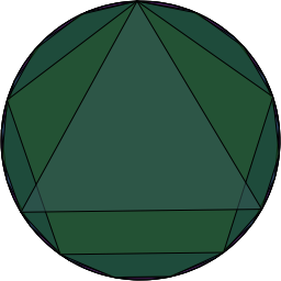
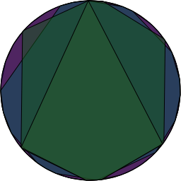
This means there are only 8 different subset of $GF(2^8)$ ‘s non-zero elements which form subgroups. Pictorially, if we placed the powers of $a$ around a circle so that $a^0 = 1$ was at the top and the powers progressed around the circle and then drew a polygon connecting consecutive points, then consecutive points in the $a^3$ sequence and consecutive points in the $a^5$ sequence, etc…. we’d end up with this:

If we don’t reorder them and just leave them in the numerical order of their binary representation, the result isn’t as aesthetically pleasing as the previous picture. Here are the same two we used before 100011011 (on the left) and 110011111 (on the right). They are easier to look at. They do not lend much more insight nor make a better stereo pair.

*shrug* Here’s the source file that I used to generate all of these images with Vecto and ZPNG: group.lisp

If it quacks like a parabola… September 21st, 2011
Patrick Stein

I am working on a game idea that involves (special) relativistic mechanics instead of classical mechanics. Working out the details that I needed was easy enough if I assumed that:

ships had a maximum speed at which they could move relative to my base frame
ships could instantly go from stopped to maximum speed or vice-versa

I didn’t like those assumptions at all. So, I started playing with the equations for relativity. In classical mechanics, the rate-of-change of velocity equals the force you’re applying divided by your mass: $\frac{dv}{dt} = \frac{F}{m}$ .

In special relativity, your mass increases with velocity. So, that equation becomes: $\frac{d\left(\frac{v}{\sqrt{1-v^2}}\right)}{dt} = \frac{F}{m_0}$ (assuming units where the speed of light is 1 unit of distance per 1 unit of time and $m_0$ is your rest-mass).

For the purposes of this post, I’m going to assume the simplest initial conditions: you start motionless and at the origin. For ease of notation, let $a = \frac{F}{m_0}$ . Solving the above differential equation to get a formula for velocity and solving the resulting differential equation to get the distance $x$ you’ve travelled in my base frame by time $t$ , the answer comes out to: $x(t) = \frac{1}{a}\left(-1 + \sqrt{1+a^2t^2}\right)$ .

I have solved this problem at least thirty times in the past two months. Sometimes I used the simple initial conditions as above. Sometimes I did it in all of its gory details (including the messy case where the applied force is not aligned with the current velocity).

I got the same answer (well, plus the extra mess when I did the full-on problem) every way that I tried it.

So, why did I do it over and over again?

If this were classical mechanics, the end equation would have been $x(t) = \frac{1}{2}at^2$ . And, I know that for low velocities, the classical mechanics answer should be almost identical to the special relativity answer. And, there was no way that I thought $\frac{1}{a}\left(-1 + \sqrt{1+a^2t^2}\right) \approx \frac{1}{2}at^2$ .

I knew what the graph $x = \sqrt{a^2t^2}$ looked like when $t \ge 0$ . It is a straight line. It doesn’t look much like the parabola $x = \frac{1}{2}a t^2$ at all.

My assumption was that since $x = \sqrt{a^2t^2}$ was a straight line for $t \ge 0$ , then $x = \sqrt{1 + a^2t^2}$ would be a straight line shifted up one unit and bent (concave-down) a little bit like the graph of $x = \sqrt{at}$ is bent.

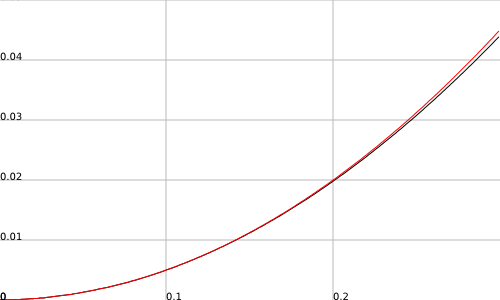
Boy was I wrong. Here is a plot of the two together (created with fooplot). The red line is the classical mechanics version. The black line is the relativistic version. Here, the force is such that the body is accelerating at a rate of the speed of light per second so they’ve already gotten up to around 28,000 miles per second before you can see any separation in the graphs here.

Definitely, I can see the resemblance. Now, to fix my intuition about square-roots.

Calculating the mean and variance with one pass February 15th, 2011
Patrick Stein

A friend showed me this about 15 years ago. I use it every time I need to calculate the variance of some data set. I always forget the exact details and have to derive it again. But, it’s easy enough to derive that it’s never a problem.

I had to derive it again on Friday and thought, I should make sure more people get this tool into their utility belts.

First, a quick refresher on what we’re talking about here. The mean $\mu$ of a data set ${ x_1, x_2, \ldots, x_n }$ is defined to be $\frac{1}{n} \sum_{i=1}^n x_i$ . The variance $\sigma^2$ is defined to be $\frac{1}{n} \sum_{i=1}^n (x_i - \mu)^2$ .

A naïve approach to calculating the variance then goes something like this:

(defun mean-variance (data)
(flet ((square (x) (* x x)))
(let* ((n (length data))
(sum (reduce #'+ data :initial-value 0))
(mu (/ sum n))
(vv (reduce #'(lambda (accum xi)
(+ accum (square (- xi mu))))
data :initial-value 0)))
(values mu (/ vv n)))))

This code runs through the data list once to count the items, once to calculate the mean, and once to calculate the variance. It is easy to see how we could count the items at the same time we are summing them. It is not as obvious how we can calculate the sum of squared terms involving the mean until we’ve calculated the mean.

If we expand the squared term and pull the constant $\mu$ outside of the summations it ends up in, we find that:

$\frac{\sum (x_i - \mu)^2}{n} = \frac{\sum x_i^2}{n} - 2 \mu \frac{\sum x_i}{n} + \mu^2 \frac{\sum 1}{n}$

When we recognize that $\frac{\sum x_i}{n} = \mu$ and $\sum_{i=1}^n 1 = n$ , we get:

$\sigma^2 = \frac{\sum x_i^2}{n} - \mu^2 = \frac{\sum x_i^2}{n} - \left( \frac{\sum x_i}{n} \right)^2$ .

This leads to the following code:

(defun mean-variance (data)
(flet ((square (x) (* x x)))
(destructuring-bind (n xs x2s)
(reduce #'(lambda (accum xi)
(list (1+ (first accum))
(+ (second accum) xi)
(+ (third accum) (square xi))))
data :initial-value '(0 0 0))
(let ((mu (/ xs n)))
(values mu (- (/ x2s n) (square mu)))))))

The code is not as simple, but you gain a great deal of flexibility. You can easily convert the above concept to continuously track the mean and variance as you iterate through an input stream. You do not have to keep data around to iterate through later. You can deal with things one sample at a time.

The same concept extends to higher-order moments, too.

Happy counting.

Edit: As many have pointed out, this isn’t the most numerically stable way to do this calculation. For my part, I was doing it with Lisp integers, so I’ve got all of the stability I could ever want. 🙂 But, yes…. if you are intending to use these numbers for big-time decision making, you probably want to look up a really stable algorithm.

nklein software

software development and consulting

Lines Are Big Circles September 13th, 2013
Patrick Stein

What is a basis?

Okay, but what is an orthonormal basis?

What about Projective and Null?

Clifford Algebras with an Orthonormal Basis

What Happens When You Don’t Have An Orthonormal Basis?

26 SLOC

Visualizing Galois Fields (Follow-up) May 21st, 2012
Patrick Stein

If it quacks like a parabola… September 21st, 2011
Patrick Stein

Calculating the mean and variance with one pass February 15th, 2011
Patrick Stein

RSS Feeds

Links

Categories

Recent Posts

Archives

nklein software

software development and consulting

Lines Are Big Circles September 13th, 2013 Patrick Stein

What is a basis?

Okay, but what is an orthonormal basis?

What about Projective and Null?

Clifford Algebras with an Orthonormal Basis

What Happens When You Don’t Have An Orthonormal Basis?

26 SLOC

Share this:

Visualizing Galois Fields (Follow-up) May 21st, 2012 Patrick Stein

Share this:

Visualizing Galois Fields May 17th, 2012 Patrick Stein

Arithmetic in Galois Fields

How is the Galois field structured?

What’s next?

Share this:

If it quacks like a parabola… September 21st, 2011 Patrick Stein

Share this:

Calculating the mean and variance with one pass February 15th, 2011 Patrick Stein

Share this:

RSS Feeds

Links

Categories

Recent Posts

Tags

Archives

Lines Are Big Circles September 13th, 2013
Patrick Stein

Visualizing Galois Fields (Follow-up) May 21st, 2012
Patrick Stein

Visualizing Galois Fields May 17th, 2012
Patrick Stein

If it quacks like a parabola… September 21st, 2011
Patrick Stein

Calculating the mean and variance with one pass February 15th, 2011
Patrick Stein