Finding the Perfect Hyperbola February 15th, 2010
Patrick Stein

For an application that I’m working on, I needed a way to scale quantities that range (theoretically) over the real numbers (though practically are probably between plus and minus three) into positive numbers. I wanted the function to be everywhere increasing, I wanted f(0) = 1, and I wanted control of the derivative at x = 0.

The easy choice is: f(x) = e^{\alpha x}. This is monotonically increasing. f(0) = 1 and f^\prime(0) = \alpha.

I needed to scale three such quantities and mush them together. I thought it’d be spiffy then to have three different functions that satisfy my criteria. The next logical choice was f(x) = 1 + \mathrm{tanh} (\alpha x). It is everywhere positive and increasing. And, it has f^\prime(0) = \alpha.

Now, I needed third function that was always positive, always increasing, had f(0) = 1 and f^\prime(0) = \alpha. One choice was: f(x) = e^{e^{\alpha x} - 1}. But, that seemed like overkill. It also meant that I really had to keep my \alpha tiny if I didn’t want to scale things into the stratosphere.

Playing with hyperbolas
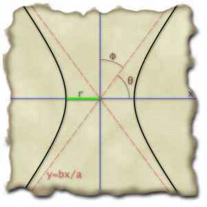
So, I thought… why don’t I make a hyperbola, rotate it, and shift it so that the apex of one side of the hyperbola is at (0,1). And, I can adjust the parameters of the hyperbola so that f'(0) = \alpha. After a variety of false starts where I tried to keep the hyperbola general until the very end (\frac{x^2}{a^2} - \frac{y^2}{b^2} = r^2, rotated by \theta degrees, and shifted by \beta), I quickly got bogged down in six or seven incredibly ugly equations in eight or nine variables.

So, it was time to start trying to make it easy from the beginning. I noticed that if was going to rotate it by an angle \theta in the clockwise direction, then I needed \phi = \frac{\pi}{2} - \theta to be such that \tan \phi = \alpha if my slope was going to work out right in the end. So, I’m looking at the basic triangle on the right then to determine all of my sines and cosines and such.
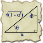
Based on that triangle, it was also obvious that the asymptote for my starting hyperbola had to have \frac{b}{a} = \frac{1}{\alpha}. I played around a bit then with making a = \alpha and b = 1. In the end, I found things simplified sooner if I started with a = 1 and b = \frac{1}{\alpha}.

I also needed r to be such that the point (-r,0) rotate up so that its y-coordinate was 1. This meant that r \sin \theta = 1 or r = \frac{1}{\sin \theta} = \sqrt{1 + \alpha^2}.

So, my starting hyperbola then was: x^2 - \alpha^2 y^2 = 1 + \alpha^2.

From there, I had to rotate the x and y by \theta in the clockwise direction. This gave me:

(x\cos\theta - y\sin\theta)^2 - \alpha^2 (x\sin\theta + y\cos\theta)^2 = 1 + \alpha^2

A little multiplying out leads to:

(x^2\cos^2\theta - 2xy\sin\theta\cos\theta + y^2\sin^2\theta) \\ - \alpha^2(x^2\sin^2\theta + 2xy\sin\theta\cos\theta + y^2\cos^2\theta) = 1 + \alpha^2

From there, using cos^2\theta = \frac{\alpha^2}{1 + \alpha^2}, sin^2\theta = \frac{1}{1 + \alpha^2}, and \sin\theta\cos\theta = \frac{\alpha}{1 + \alpha^2}, we come to:

\frac{-2\alpha(1 + \alpha^2)xy + ( 1 - \alpha^4 )y^2}{1 + \alpha^2} = -2\alpha{}xy +  (1 - \alpha^2)y^2 = 1 + \alpha^2

The only step remaining was to shift it all over so that when y = 1, we end up with x = 0. Plugging in y = 1, we see that -2x\alpha + 1 - \alpha^2 = 1 + \alpha. That equation balances when x = -\alpha. We want it to balance when x = 0, so we’re going to substitute (x - \alpha) in place of the x in the above equation to get:

-2\alpha(x - \alpha)y + (1 - \alpha^2)y^2 = 1 + \alpha^2

We can easily verify that the point (0,1) is on the curve. And, we can implicitly differentiate the above to get:

-2\alpha(x - \alpha)\frac{dy}{dx} - 2\alpha{}y + 2(1 - \alpha^2)y\frac{dy}{dx} = 0

Plopping x = 0 and y = 1 in there, we find that \frac{dy}{dx} = \alpha.

This is pretty good as it goes. The only step is to complete the square to find a nicer expression for y in terms of x. We start by adding \left[ \frac{\alpha}{\sqrt{1 - \alpha^2}} (x - \alpha) \right]^2 to both sides to get:

\left[ \sqrt(1 - \alpha^2)y - \frac{\alpha}{\sqrt{1 - \alpha^2}(x - \alpha)} \right]^2 = 1 + \alpha^2 + \frac{\alpha}{1 - \alpha^2} (x-\alpha)^2

This is easy enough to solve for y by taking the square root of both sides and shuffling some things about:

y = \frac{\alpha}{1 - \alpha^2}(x - \alpha) + \frac{1}{\sqrt{1 - \alpha^2}} \sqrt{1 + \alpha^2 + \frac{\alpha^2}{1 - \alpha^2}(x - \alpha)^2}

Here are all three curves with \alpha = \frac{1}{4}. The exponential is in black, the hyperbolic tangent is in red, and the hyperbola is in blue:
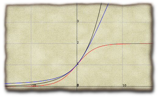
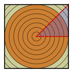
The first image on the page here was made with Zach’s Vecto library with some post-processing in the GIMP. (Here is the source file: hyperbola.lisp.) The second image was made entirely within the GIMP. And, the last image was made using Foo Plot and the GIMP.

DSL for Drawing Floor Plans October 28th, 2009
Patrick Stein

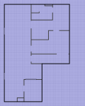
Last week, I needed create a scale drawing of my basement floor plan. My license for OmniGraffle Professional are long since out-of-date. I didn’t want to pay $200 for a new license or even another $75 if I can dig up one of my old license keys. So, what’s a hacker to do? Roll his own (on top of Zach’s Vecto library).

My first cut worked, but was pretty ugly:

(with-floor-plan #P"basement.png" 200.0
   (interior-wall :start (cons (- 91 31 1/2) 0) ; hose cover
                  :north 18
                  :east  (+ 31 1/2))
   (interior-wall :start (cons 91 (- 103 27 30)) ; storage wall
                  :south (- 103 27 30))
   (interior-wall :start (cons (+ 91 83) 103)  ; fish-tank wall
                  :to '(91 . 103)
                  :south 27)
   ...)

basement
I ended up with large calculations like that (- 103 27 30) you see there. It worked. I got an okay looking floor-plan out of it. But, it was obvious that it needed some rethinking.

My next thought was turtle graphics! Tell things where to move. Tell it to start drawing an interior wall. Tell it where to move. Tell it to start drawing a window. Tell it where to move. Tell it to stop drawing a window. Etc. This has possibilities, especially for an internal representation (which I need because I want to autoscale the drawing to fit on a sheet of paper well, so I can’t start drawing until I’ve determined the extents). However, it seems awkward to go with all of the start/stop commands. I am thinking of going more in this sort of direction:

;; The floor-plan stuff works in units.  To facility readability, I am
;; going to make some simple functions that use feet and inches instead
;; of units.  If you want centimeters and meters, go for it.

(flet ((feet (n) (* n 12))
       (inches (n) n))
  (with-floor-plan (#P"floor-plan.png"
                      :max-width       8.0  ; maximum width of output (units)
                      :max-height     10.0  ; maximum height of output (units)
                      :dots-per-unit 300.0  ; resolution of output
                      :grid     (inches 6)) ; size of background-grid

    (compass :north 180.0)   ; draw north indication 180 degrees CCW from right

    (exterior-wall         ; start drawing an exterior wall
       :closed t           ; that closes at the end
       (left (feet 10))    ; extend wall left 10 feet
       (up (feet 6))       ; extend wall up 6 feet
       (window
          (up (inches 30))) ; draw 30" window
       (up (inches 8))      ; draw 8" wall
       (door :starts :hinge-side      ; or :latch-side
             :opens :left             ; or :right seen from direction of motion
             (up (inches 30)))        ; this door goes up, so :left is to
                                      ; the left of the page
       (up (inches 8))
       (right (feet 10)))

    (left (feet 4))                    ; move four feet to the left
    (interior-wall
       (up (feet 5))
       (right (inches 8))
       (door :starts :latch-side
             :opens :right
             (right (inches 30)))
       (right-to (feet 0)))            ; move to an absolute left-right coordinate
    (move (feet 2) (feet (+ 2 1/2)))
    (label "Bathroom")))

Has anyone tackled this problem well already? Or, have any suggestions of how to improve this?

Ask a simple question… August 8th, 2009
Patrick Stein

Ask a simple question, spend the next forty minutes sifting through integral tables. Earlier, I took some code that was uniformly selecting points from a square centered at the origin and converted it to code using points from a normal distribution. For my purposes, I used a standard-deviation for the normal distribution that was half of the in-radius of the box. It wasn’t at all exact in any way.

What if I wanted to be exact? Suppose I wanted to switch from points uniformly distributed in a box to points from a normal distribution while maintaining the expected distance from the selected point to the origin.

What exactly is the expected distance from a selected point to the origin if one picks each coordinate for the point from a uniform distribution on the range [-1,+1]? Let’s start with the one-dimensional case. The probability density is \frac{1}{2} everywhere. So, the answer is 2 \int_{r=0}^1 \frac{1}{2} r dr = \frac{1}{2} as we would expect.

(image created in Lisp using Zach's Vecto library)How about two dimensions? This is immediately more awkward. The one-dimensional disk looks exactly like the one-dimensional square. In two dimensions, the disk and square are quite different. We either have to integrate over the square and calculate the radius of each point, or we have to integrate over increasing radii and be careful once we get to the in-radius of the square. (image created in Lisp using Zach's Vecto library)

I originally chose to try to integrate over the square. The probability density is \frac{1}{4} everywhere. This means the expected radius is \int_{y=-1}^1 \int_{x=-1}^1 \sqrt{x^2+y^2} dx dy. This gets to be no fun very fast since the inner integral comes out with a logarithm in it. I mean, do you want to finish this integral?

\int_{y=-1}^1 \left.\left( \frac{1}{2} x \sqrt{x^2 + y^2} + \frac{1}{2} y^2 \ln \left( x + \sqrt{x^2 + y^2} \right)\right)\right|_{x=-1}^1 dy

It may be easy. I didn’t want to mess with it. I suppose once you evaluate the x terms, it reduces a fair bit (if I did that all right):
\int_{y=-1}^1 \left( \sqrt{1 + y^2} + \frac{1}{2} y^2 \ln \left( \frac{1 + \sqrt{1 + y^2}}{-1 + \sqrt{1 + y^2}} \right) \right) dy

I still don’t want to touch it.

So, how about integrating over the radii? Again, the probability density is \frac{1}{4} everywhere. This makes the expected radius:

\int_{r=0}^1 \frac{1}{4} \cdot 2 \pi r dr + \int_{r=1}^{\sqrt{2}} \frac{1}{4} \cdot 8 \left( \frac{\pi}{4} - \arccos \frac{1}{r} \right) dr

With a little massaging, you can move the \frac{\pi}{4} from the second integral into the first instead:
\int_{r=0}^{\sqrt{2}} \frac{1}{4} \cdot 2 \pi r dr - \int_{r=1}^{\sqrt{2}} \frac{1}{4} \cdot 8 \arccos \frac{1}{r} dr

This is hardly consolation though. Here is where we get lost in our table of integrals for the better part of an hour.

And, this is only the two-dimensional case! In my original problem, the ambient space was 32-dimensional. My, oh my.

l